Statistics and Probability
Welcome to Our Site
I greet you this day,
These are the solutions to the Cambridge IGCSE (International General Certificate of Secondary Education)
past questions on Statistics and Probability.
The link to the video solutions will be provided for you. Please subscribe to the YouTube channel to be notified
of upcoming livestreams.
You are welcome to ask questions during the video livestreams.
If you find these resources valuable and if any of these resources were helpful in your passing the
any of the Cambridge Assessments on Mathematics, please consider making a donation:
Cash App: $ExamsSuccess or
cash.app/ExamsSuccess
PayPal: @ExamsSuccess or
PayPal.me/ExamsSuccess
Google charges me for the hosting of this website and my other
educational websites. It does not host any of the websites for free.
Besides, I spend a lot of time to type the questions and the solutions well.
As you probably know, I provide clear explanations on the solutions.
Your donation is appreciated.
Comments, ideas, areas of improvement, questions, and constructive criticisms are welcome.
Feel free to contact me. Please be positive in your message.
I wish you the best.
Thank you.
-
Symbols and Meanings
- $X$ = dataset $X$
- $x = x-values$ OR data values
- $x_{mid}$ = class midpoint of $x-values$ = class midpoint of the data values
- $\Sigma$ (pronounced as uppercase Sigma) = $summation$
- $\Sigma x$ = summation of the $x-values$
- $f = frequency$
- $F = frequency$
- $\Sigma f$ = summation of the frequencies
- $\Sigma fx$ = summation of the product of the $x-values$ and their corresponding frequencies
- $(\Sigma x)^2$ = square of the summation of the $x-values$
- $\Sigma x^2$ = summation of the squared of the $x-values$
- $\bar{x}$ is sample mean of the $x-values$
- $\mu$ = population mean
- $n$ = sample size
- $N$ = population size
- $\tilde{x}$ = median
- $\widehat{x}$ = mode
- $AM$ = assumed mean
- $D$ = deviation from the assumed mean
- $x_{MR}$ = midrange
- $LCL$ = lower class limit
- $UCL$ = upper class limit
- $min$ = minimum data value
- $max$ = maximum data value
- $LCB_{med}$ = lower class boundary of the median class
- $CW$ = class width
- $f_{med}$ = frequency of the median class
- $CF_{bmed}$ = cumulative frequency of the class before the median class
- $LCB_{mod}$ = lower class boundary of the modal class
- $f_{mod}$ = frequency of the modal class
- $f_{bmod}$ = frequency of the class before the modal class
- $f_{amod}$ = frequency of the class after the modal class
- $R$ = range
- $s$ = sample standard deviation
- $s^2$ = sample variance
- $\sigma$ = population standard deviation
- $\sigma^2$ = population variance
- $CV$ = coefficient of variation
- $z = z-score$
- $Q_1$ = lower quartile or first quartile
- $P_{25}$ = 25th percentile or first quartile
- $Q_2$ = middle quartile or second quartile or median
- $P_{50}$ = 50th percentile or median
- $Q_3$ = upper quartile or third quartile
- $P_{75}$ = 75th percentile or third quartile
- $IQR$ = interquartile range
- $SIQR$ = semi-interquartile range
- $MQ$ = midquartile
- $LF$ = lower fence
- $UF$ = upper fence
- $TM$ = trimmed mean
- $\Pi$ (pronounced as uppercase Pi) = $product$
- $\Pi x$ = product of the $x-values$
- $GM$ = geometric mean
Grouped Data
$
\underline{\text{Class Size or Class Width}} \\[3ex]
(1.)\;\; Class\:\:Width = \dfrac{Maximum - Minimum}{Number\:\:of\:\:classes} \\[5ex]
(2.)\;\; Class\:\:Width = LCI\:\:of\:\:2nd\:\:Class - LCI\:\:of\:\:1st\:\:Class \\[3ex]
(3.)\;\; Class\:\:Width = UCI\:\:of\:\:2nd\:\:Class - UCI\:\:of\:\:1st\:\:Class \\[3ex]
(4.)\;\; Class\:\:Width = UCB\:\:of\:\:a\:\:class - LCB\:\:of\:\:the\:\:same\:\:class \\[3ex]
(5.)\;\; Class\:\:Width = LCB\:\:of\:\:a\:\:Class - LCB\:\:of\:\:previous\:\:class \\[5ex]
\underline{\text{Frequency Density}} \\[3ex]
(6.)\;\; \text{Frequency Density} = \dfrac{\text{Frequency}}{\text{Class Width}} \\[7ex]
\underline{\text{Class Midpoints or Class Marks}} \\[3ex]
(7.)\;\; Class\:\:Width = LCB\:\:of\:\:a\:\:Class - LCB\:\:of\:\:previous\:\:class \\[5ex]
\underline{\text{Class Boundaries}} \\[3ex]
(8.)\;\; Lower\:\:Class\:\:Boundary\:\:of\:\:a\:\:class = \dfrac{LCI\:\:of\:\:that\:\:class +
UCI\:\:of\:\:previous/preceding\:\:class}{2} \\[5ex]
(9.)\;\; Upper\:\:Class\:\:Boundary\:\:of\:\:a\:\:class = \dfrac{UCI\:\:of\:\:that\:\:class +
LCI\:\:of\:\:next/succeeding\:\:class}{2} \\[5ex]
$
(10.) Shortcut for Class Boundaries
If the class intervals are integers:
Lower Class Boundary = Lower Class Interval − 0.5
Upper Class Boundary = Upper Class Interval + 0.5
If the class intervals are decimals in one decimal place:
Lower Class Boundary = Lower Class Interval − 0.05
Upper Class Boundary = Upper Class Interval + 0.05
If the class intervals are decimals in two decimal places:
Lower Class Boundary = Lower Class Interval − 0.005
Upper Class Boundary = Upper Class Interval + 0.005
...and so on and so forth.
$
\underline{\text{Relative Frequency}} \\[3ex]
(11.)\;\; RF\:\:of\:\:a\:\:class = \dfrac{Frequency\:\:of\:\:that\:\:class}{\Sigma Frequency} \\[7ex]
\underline{\text{Cumulative Frequency}} \\[3ex]
(12.)\;\; CF\:\:of\:\:1st\:\:Class = Frequency\:\:of\:\:1st\:\:Class \\[3ex]
CF\:\:of\:\:2nd\:\:Class = Frequency\:\:of\:\:1st\:\:Class + Frequency\:\:of\:\:2nd\:\:Class \\[3ex]
CF\:\:of\:\:3rd\:\:Class = Frequency\:\:of\:\:1st\:\:Class + Frequency\:\:of\:\:2nd\:\:Class +
Frequency\:\:of\:\:3rd\:\:Class \\[3ex]
CF = CF\:\:of\:\:Last\:\:Class = \Sigma Frequency
$
Measures of Center: Raw Data and Ungrouped Data
$ \underline{Sample\:\:Mean} \\[3ex] (1.)\:\: \bar{x} = \dfrac{\Sigma x}{n} \\[5ex] (2.)\:\: n = \Sigma f \\[3ex] (3.)\:\: \bar{x} = \dfrac{\Sigma fx}{\Sigma f} \\[5ex] \underline{Given\:\:an\:\:Assumed\:\:Mean} \\[3ex] (4.)\:\: D = x - AM \\[3ex] (5.)\:\: \bar{x} = AM + \dfrac{\Sigma D}{n} \\[5ex] (6.)\:\: \bar{x} = AM + \dfrac{\Sigma fD}{\Sigma f} \\[7ex] \underline{Population\:\:Mean} \\[3ex] (7.)\:\: \mu = \dfrac{\Sigma x}{N} \\[5ex] (8.)\:\: N = \Sigma f \\[3ex] \underline{Given\:\:an\:\:Assumed\:\:Mean} \\[3ex] (9.)\:\: D = x - AM \\[3ex] (10.)\:\: \mu = AM + \dfrac{\Sigma D}{N} \\[5ex] (11.)\:\: \mu = AM + \dfrac{\Sigma fD}{\Sigma f} \\[7ex] \underline{Median} \\[3ex] (12.)\:\: \tilde{x} = \left(\dfrac{\Sigma f + 1}{2}\right)th \:\:for\:\:sorted\:\:odd\:\:sample\:\:size \\[5ex] (13.)\:\: \tilde{x} = \left(\dfrac{\Sigma f}{2}\right)th \:\:for\:\:sorted\:\:even\:\:sample\:\:size \\[7ex] \underline{Mode} \\[3ex] (14.)\:\: Mode = x-value(s) \:\;with\:\:highest\:\:frequency \\[5ex] \underline{Midrange} \\[3ex] (15.)\:\: x_{MR} = \dfrac{min + max}{2} \\[5ex] \underline{Geometric\;\;Mean} \\[3ex] (16.)\;\; GM = \sqrt[n]{\prod\limits_{x=1}^n x} $
Measures of Center: Grouped Data
$ \underline{Class\:\:Midpoint} \\[3ex] (1.)\:\: x_{mid} = \dfrac{LCL + UCL}{2} \\[7ex] Equal\:\:Class\:\:Intervals\:(Same\:\:Class\:\:Size) \\[3ex] \underline{Mean} \\[3ex] (2.)\:\: \bar{x} = \dfrac{\Sigma fx_{mid}}{\Sigma f} \\[7ex] Equal\:\:Class\:\:Intervals\:(Same\:\:Class\:\:Size) \\[3ex] \underline{Given\:\:an\:\:Assumed\:\:Mean} \\[3ex] (3.)\:\: D = x_{mid} - AM \\[3ex] (4.)\:\: \bar{x} = AM + \dfrac{\Sigma fD}{\Sigma f} \\[7ex] \underline{Median} \\[3ex] (5.)\:\: \tilde{x} = LCB_{med} + \dfrac{CW}{f_{med}} * \left[\left(\dfrac{\Sigma f}{2}\right) - CF_{bmed}\right] \\[7ex] \underline{Mode} \\[3ex] (6.)\:\: \widehat{x} = LCB_{mod} + CW * \left[\dfrac{f_{mod} - f_{bmod}}{(f_{mod} - f_{bmod}) + (f_{mod} - f_{amod})}\right] $
Measures of Spread: Raw Data and Ungrouped Data
$ \underline{Range} \\[3ex] (1.)\:\: Range = max - min \\[3ex] \underline{Using\;\;Assumed\;\;Mean} \\[3ex] (2.)\;\; D = x - AM \\[5ex] \underline{Sample\:\:Variance} \\[3ex] \color{red}{First\:\:Formula} \\[3ex] (3.)\:\: s^2 = \dfrac{\Sigma(x - \bar{x})^2}{n - 1} \\[5ex] (4.)\:\: s^2 = \dfrac{\Sigma f(x - \bar{x})^2}{\Sigma f - 1} \\[5ex] \color{red}{Second\:\:Formula} \\[3ex] (5.)\:\: s^2 = \dfrac{n(\Sigma x^2) - (\Sigma x)^2}{n(n - 1)} \\[5ex] (6.)\:\: s^2 = \dfrac{\Sigma f(\Sigma fx^2) - (\Sigma fx)^2}{\Sigma f(\Sigma f - 1)} \\[7ex] \underline{Using\;\;Assumed\;\;Mean} \\[3ex] (7.)\;\; s^2 = \dfrac{\Sigma D^2}{n - 1} - \left(\dfrac{\Sigma D}{n - 1}\right)^2 \\[7ex] (8.)\;\; s^2 = \dfrac{\Sigma fD^2}{\Sigma f - 1} - \left(\dfrac{\Sigma fD}{\Sigma f - 1}\right)^2 \\[10ex] \underline{Population\:\:Variance} \\[3ex] \color{red}{First\:\:Formula} \\[3ex] (9.)\:\: \sigma^2 = \dfrac{\Sigma(x - \mu)^2}{N} \\[5ex] (10.)\:\: \sigma^2 = \dfrac{\Sigma f(x - \mu)^2}{\Sigma f} \\[5ex] \color{red}{Second\:\:Formula} \\[3ex] (11.)\:\: \sigma^2 = \dfrac{N(\Sigma x^2) - (\Sigma x)^2}{N^2} \\[5ex] (12.)\:\: \sigma^2 = \dfrac{\Sigma f(\Sigma fx^2) - (\Sigma fx)^2}{(\Sigma f)^2} \\[7ex] \underline{Using\;\;Assumed\;\;Mean} \\[3ex] (13.)\;\; \sigma^2 = \dfrac{\Sigma D^2}{N} - \left(\dfrac{\Sigma D}{N}\right)^2 \\[7ex] (14.)\;\; \sigma^2 = \dfrac{\Sigma fD^2}{\Sigma f} - \left(\dfrac{\Sigma fD}{\Sigma f}\right)^2 \\[10ex] \underline{Sample\:\:Standard\:\:Deviation} \\[3ex] \color{red}{First\:\:Formula} \\[3ex] (15.)\:\: s = \sqrt{\dfrac{\Sigma(x - \bar{x})^2}{n - 1}} \\[5ex] (16.)\:\: s = \sqrt{\dfrac{\Sigma f(x - \bar{x})^2}{\Sigma f - 1}} \\[5ex] \color{red}{Second\:\:Formula} \\[3ex] (17.)\:\: s = \sqrt{\dfrac{n(\Sigma x^2) - (\Sigma x)^2}{n(n - 1)}} \\[5ex] (18.)\:\: s = \sqrt{\dfrac{\Sigma f(\Sigma fx^2) - (\Sigma fx)^2}{\Sigma f(\Sigma f - 1)}} \\[7ex] \underline{Using\;\;Assumed\;\;Mean} \\[3ex] (19.)\;\; s = \sqrt{\dfrac{\Sigma D^2}{n - 1} - \left(\dfrac{\Sigma D}{n - 1}\right)^2} \\[7ex] (20.)\;\; s = \sqrt{\dfrac{\Sigma fD^2}{\Sigma f - 1} - \left(\dfrac{\Sigma fD}{\Sigma f - 1}\right)^2} \\[10ex] \underline{Population\:\:Standard\:\:Deviation} \\[3ex] \color{red}{First\:\:Formula} \\[3ex] (21.)\:\: \sigma = \sqrt{\dfrac{\Sigma(x - \mu)^2}{N}} \\[5ex] (22.)\:\: \sigma = \sqrt{\dfrac{\Sigma f(x - \mu)^2}{\Sigma f}} \\[5ex] \color{red}{Second\:\:Formula} \\[3ex] (23.)\:\: \sigma = \dfrac{\sqrt{N(\Sigma x^2) - (\Sigma x)^2}}{N} \\[5ex] (24.)\:\: \sigma = \dfrac{\sqrt{\Sigma f(\Sigma fx^2) - (\Sigma fx)^2}}{\Sigma f} \\[7ex] \underline{Using\;\;Assumed\;\;Mean} \\[3ex] (25.)\;\; \sigma = \sqrt{\dfrac{\Sigma D^2}{N} - \left(\dfrac{\Sigma D}{N}\right)^2} \\[7ex] (26.)\;\; \sigma = \sqrt{\dfrac{\Sigma fD^2}{\Sigma f} - \left(\dfrac{\Sigma fD}{\Sigma f}\right)^2} \\[10ex] \underline{Range\:\:Rule\:\:of\:\:Thumb} \\[3ex] Approximate\:\:Value\:\:of\:\:Calculating\:\:Standard\:\:Deviation \\[3ex] (27.)\:\: s = \dfrac{Range}{4} = \dfrac{max - min}{4} \\[7ex] \underline{Interquartile\:\:Range} \\[3ex] (28.)\:\: IQR = Q_3 - Q_1 \\[5ex] \underline{Coefficient\:\:of\:\:Variation\:\:for\:\:Sample} \\[3ex] (29.)\:\: CV = \dfrac{s}{x} * 100 ...in\:\:\% \\[7ex] \underline{Coefficient\:\:of\:\:Variation\:\:for\:\:Population} \\[3ex] (30.)\:\: CV = \dfrac{\sigma}{x} * 100 ...in\:\:\% \\[7ex] \underline{Mean\:\:Absolute\:\:Deviation} \\[3ex] (31.)\:\: MAD = \dfrac{\Sigma |x - \bar{x}|}{n} \\[5ex] \underline{Mean\:\:Absolute\:\:Deviation} \\[3ex] (32.)\:\: MAD = \dfrac{\Sigma f|x - \bar{x}|}{\Sigma f} \\[5ex] $
Measures of Spread: Grouped Data
$ \underline{Class\:\:Midpoint} \\[3ex] (1.)\:\: x_{mid} = \dfrac{LCL + UCL}{2} \\[5ex] \underline{Using\;\;Assumed\;\;Mean} \\[3ex] (2.)\;\; D = x_{mid} - AM \\[5ex] \underline{Sample\:\:Variance} \\[3ex] \color{red}{First\:\:Formula} \\[3ex] (3.)\:\: s^2 = \dfrac{\Sigma f(x_{mid} - \bar{x})^2}{\Sigma f - 1} \\[5ex] \color{red}{Second\:\:Formula} \\[3ex] (4.)\:\: s^2 = \dfrac{\Sigma f(\Sigma fx_{mid}^2) - (\Sigma fx_{mid})^2}{\Sigma f(\Sigma f - 1)} \\[5ex] \underline{Using\;\;Assumed\;\;Mean} \\[3ex] (5.)\;\; s^2 = \dfrac{\Sigma D^2}{n - 1} - \left(\dfrac{\Sigma D}{n - 1}\right)^2 \\[7ex] (6.)\;\; s^2 = \dfrac{\Sigma fD^2}{\Sigma f - 1} - \left(\dfrac{\Sigma fD}{\Sigma f - 1}\right)^2 \\[10ex] \underline{Sample\:\:Standard\:\:Deviation} \\[3ex] \color{red}{First\:\:Formula} \\[3ex] (7.)\:\: s = \sqrt{\dfrac{\Sigma f(x_{mid} - \bar{x})^2}{\Sigma f - 1}} \\[5ex] \color{red}{Second\:\:Formula} \\[3ex] (8.)\:\: s = \sqrt{\dfrac{\Sigma f(\Sigma fx_{mid}^2) - (\Sigma fx_{mid})^2}{\Sigma f(\Sigma f - 1)}} \\[5ex] \underline{Using\;\;Assumed\;\;Mean} \\[3ex] (9.)\;\; s = \sqrt{\dfrac{\Sigma D^2}{n} - \left(\dfrac{\Sigma D}{n - 1}\right)^2} \\[7ex] (10.)\;\; s = \sqrt{\dfrac{\Sigma fD^2}{\Sigma f - 1} - \left(\dfrac{\Sigma fD}{\Sigma f - 1}\right)^2} \\[10ex] \underline{Population\:\:Variance} \\[3ex] \color{red}{First\:\:Formula} \\[3ex] (11.)\:\: \sigma^2 = \dfrac{\Sigma f(x_{mid} - \bar{x})^2}{\Sigma f} \\[5ex] \color{red}{Second\:\:Formula} \\[3ex] (12.)\:\: \sigma^2 = \dfrac{\Sigma f(\Sigma fx_{mid}^2) - (\Sigma fx_{mid})^2}{\Sigma f(\Sigma f)} \\[5ex] \underline{Using\;\;Assumed\;\;Mean} \\[3ex] (13.)\;\; \sigma^2 = \dfrac{\Sigma D^2}{N} - \left(\dfrac{\Sigma D}{N}\right)^2 \\[7ex] (14.)\;\; \sigma^2 = \dfrac{\Sigma fD^2}{\Sigma f} - \left(\dfrac{\Sigma fD}{\Sigma f}\right)^2 \\[10ex] \underline{Population\:\:Standard\:\:Deviation} \\[3ex] \color{red}{First\:\:Formula} \\[3ex] (15.)\:\: \sigma = \sqrt{\dfrac{\Sigma f(x_{mid} - \bar{x})^2}{\Sigma f}} \\[5ex] \color{red}{Second\:\:Formula} \\[3ex] (16.)\:\: \sigma = \sqrt{\dfrac{\Sigma f(\Sigma fx_{mid}^2) - (\Sigma fx_{mid})^2}{\Sigma f(\Sigma f)}} \\[5ex] \underline{Using\;\;Assumed\;\;Mean} \\[3ex] (17.)\;\; \sigma = \sqrt{\dfrac{\Sigma D^2}{N} - \left(\dfrac{\Sigma D}{N}\right)^2} \\[7ex] (18.)\;\; \sigma = \sqrt{\dfrac{\Sigma fD^2}{\Sigma f} - \left(\dfrac{\Sigma fD}{\Sigma f}\right)^2} \\[10ex] $
Measures of Position
A data value is usual if $-2.00 \le z-score \le 2.00$
A data value is unusual if $z-score \lt -2.00$ OR $z-score \gt 2.00$
$
\underline{Sample} \\[3ex]
Minimum\:\:usual\:\:data\:\:value = \bar{x} - 2s \\[3ex]
Maximum\:\:usual\:\:data\:\:value = \bar{x} + 2s \\[5ex]
\underline{Population} \\[3ex]
Minimum\:\:usual\:\:data\:\:value = \mu - 2\sigma \\[3ex]
Maximum\:\:usual\:\:data\:\:value = \mu + 2\sigma \\[5ex]
\underline{z\:\:score\:\:for\:\:Sample} \\[3ex]
(1.)\:\: z = \dfrac{x - \bar{x}}{s} \\[7ex]
\underline{z\:\:score\:\:for\:\:Population} \\[3ex]
(2.)\:\: z = \dfrac{x - \mu}{\sigma} \\[7ex]
\underline{Quantiles(Percentiles,\:Deciles,\:Quintiles,\:and\:Quartiles)} \\[3ex]
\color{red}{Convert\:\:a\:\:Data\:\:value\:\:to\:\:a\:\:Quantile} \\[3ex]
x\:\:and\:\:y\:\:are\:\:two\:\:different\:\:variables \\[3ex]
(3.)\:\: Percentile\:\:of\:\:x =
\dfrac{number\:\:of\:\:values\:\:less\:\:than\:\:x}{total\:\:number\:\:of\:\:values} * 100 = yth\:\:Percentile
\\[5ex]
(4.)\:\: Decile\:\:of\:\:x =
\dfrac{number\:\:of\:\:values\:\:less\:\:than\:\:x}{total\:\:number\:\:of\:\:values} * 10 = yth\:\:Decile
\\[5ex]
(5.)\:\: Quintile\:\:of\:\:x =
\dfrac{number\:\:of\:\:values\:\:less\:\:than\:\:x}{total\:\:number\:\:of\:\:values} * 5 = yth\:\:Quintile
\\[5ex]
(6.)\:\: Quartile\:\:of\:\:x =
\dfrac{number\:\:of\:\:values\:\:less\:\:than\:\:x}{total\:\:number\:\:of\:\:values} * 4 = yth\:\:Quartile
\\[7ex]
\color{red}{Convert\:\:a\:\:Quantile\:\:to\:\:a\:\:Data\:\:Value} \\[3ex]
Calculate\:\:the\:\:xth\:\:position\:\:of\:\:the\:\:yth\:\:Quantile \\[3ex]
(7.)\:\: xth\:\:position = \dfrac{yth\:\:Percentile}{100} * total\:\:number\:\:of\:\:values \\[5ex]
(8.)\:\: xth\:\:position = \dfrac{yth\:\:Decile}{10} * total\:\:number\:\:of\:\:values \\[5ex]
(9.)\:\: xth\:\:position = \dfrac{yth\:\:Quintile}{5} * total\:\:number\:\:of\:\:values \\[5ex]
(10.)\:\: xth\:\:position = \dfrac{yth\:\:Quartile}{4} * total\:\:number\:\:of\:\:values \\[7ex]
$
| If the $xth$ position | then, |
|---|---|
| is an integer |
$xth\:\:position = \dfrac{xth\:\:position + (x + 1)th\:\;position}{2}$ In other words, find the value of the $xth$ position; find the value of the next position; and determine the mean of the two values. |
| is not an integer | $xth$ position is rounded up |
$ \underline{The\:\:Five-Number\:\:Summary\:\:of\:\:Data} \\[3ex] (11.)\:\: Minimum\:(min) \\[3ex] (12.)\:\: Lower\:\:Quartile\:(Q_1) \\[3ex] (13.)\:\: Median\:\:or\:\:Middle\:\:Quartile\:(Q_2) \\[3ex] (14.)\:\: Upper\:\:Quartile\:(Q_3) \\[3ex] (15.)\:\: Maximum\:(Max) \\[5ex] \underline{Other\:\:Statistics\:\:from\:\:Quantiles} \\[3ex] (16.)\:\: IQR = Q_3 - Q_1 \\[3ex] (17.)\:\: SIQR = \dfrac{IQR}{2} = \dfrac{Q_3 - Q_1}{2} \\[5ex] (18.)\:\: MQ = \dfrac{Q_3 + Q_1}{2} \\[5ex] (19.)\:\: Upper\:\:Quartile\:(Q_3) \\[3ex] (20.)\:\: LF = Q_1 - 1.5(IQR) \\[3ex] (21.)\:\: UF = Q_3 + 1.5(IQR) $
Probability
Given any two events say A and B
$
P(E) = \dfrac{n(E)}{n(S)} \\[5ex]
\underline{\text{Addition Rule}} \\[3ex]
\dfrac{n(A \cup B)}{n(S)} = \dfrac{n(A)}{n(S)} + \dfrac{n(B)}{n(S)} - \dfrac{n(A \cap B)}{n(S)} \\[5ex]
P(A \cup B) = P(A) + P(B) - P(A \cap B) \\[3ex]
P(A\:\:\:OR\:\:\:B) = P(A) + P(B) - P(A\:\:\:AND\:\:\:B) \\[5ex]
$
For Independent Events
$
P(B|A) = P(B) \\[3ex]
\rightarrow P(A\:\:\:OR\:\:\:B) = P(A) + P(B) - [P(A) * P(B)] \\[5ex]
$
For Dependent Events
$
P(B|A) = P(B|A) \\[3ex]
\rightarrow P(A\:\:\:OR\:\:\:B) = P(A) + P(B) - [P(A) * P(B|A)] \\[5ex]
$
For Mutually Exclusive Events (Disjoint Events)
$
P(A \cap B) = 0 \\[3ex]
P(A\:\:\:OR\:\:\:B) = P(A) + P(B) - 0 \\[3ex]
\rightarrow P(A\:\:\:OR\:\:\:B) = P(A) + P(B) \\[5ex]
$
$
\underline{\text{Multiplication Rule}} \\[3ex]
P(A\:\:\:AND\:\:\:B) = P(A) * P(B|A) \\[3ex]
P(A \cap B) = P(A) * P(B|A) \\[3ex]
P(A\:\:\:AND\:\:\:B) = P(A \cap B) \\[5ex]
$
$P(B|A)$ is read as: the probability of event $B$ given event $A$
For Independent Events
$
P(B|A) = P(B) \\[3ex]
\rightarrow P(A\:\:\:AND\:\:\:B) = P(A) * P(B) \\[5ex]
$
For Dependent Events
$
P(B|A) = P(B|A) \\[3ex]
\rightarrow P(A\:\:\:AND\:\:\:B) = P(A) * P(B|A) \\[5ex]
$
The complement of Event $A$ is $A'$
$
\underline{Complementary\;\;Rule} \\[3ex]
P(A) + P(A') = 1 \\[3ex]
\rightarrow P(A') = 1 - P(A) \\[5ex]
$
Other Formulas
$
(1.)\;\; P(A) = P(A \cap B') + P(A \cap B)
$
Probability Distributions
$
\boldsymbol{Probability\;\;Distribution} \\[3ex]
(1.)\;\;\mu = \Sigma[x * P(x)] \\[3ex]
(2.)\;\;E = \Sigma[x * P(x)] \\[3ex]
(3.)\;\; \sigma = \sqrt{\Sigma[x^2 * P(x)] - \mu^2} \\[7ex]
\boldsymbol{Combinatorics} \\[3ex]
(1.)\:\: 0! = 1 \\[3ex]
(2.)\:\: n! = n * (n - 1) * (n - 2) * (n - 3) * ... * 1 \\[3ex]
(3.)\;\; n! = n * (n - 1)! \\[3ex]
(4.)\;\; n! = (n - 1) * (n - 2)!...among\;\;others \\[3ex]
(5.)\:\: C(n, x) = \dfrac{n!}{(n - x)!x!} \\[5ex]
(6.)\;\; C(n, x) = C(n, n - x) \\[7ex]
\boldsymbol{Binomial\;\;Distribution} \\[3ex]
(1.)\;\; p + q = 1 \\[3ex]
(2.)\;\; \mu = n * p \\[3ex]
(3.)\;\; \sigma = \sqrt{n * p * q} \\[4ex]
(4.)\;\; P(x) = C(n, x) * p^x * q^{n - x}...\text{Depends on the context of the question} \\[5ex]
where \\[3ex]
x = \text{number of successes/failures} \\[3ex]
n = \text{number of trials} = 12 \\[3ex]
C(n, x) = \text{Binomial coefficient} \\[3ex]
P(x) = \text{Probability of the number of successes/failures} \\[3ex]
p = \text{probability of success} \\[3ex]
q = \text{probability of failure} \\[5ex]
\boldsymbol{Poisson\;\;Distribution} \\[3ex]
(1.)\;\;P(x) = \dfrac{\mu^x * e^{-\mu}}{x!} \\[5ex]
(2.)\;\; \mu = \sigma^2 \\[7ex]
\boldsymbol{Normal\;\;Distribution} \\[3ex]
(1.)\;\; z = \dfrac{x - \bar{x}}{s} \\[5ex]
(2.)\;\; x = \bar{x} + zs \\[3ex]
(3.)\;\; z = \dfrac{x - \mu}{\sigma} \\[5ex]
(4.)\;\; x = \mu + z\sigma \\[3ex]
(5.)\;\;\text{Probability Density Function},\;\;P(x) =
\dfrac{1}{\sigma\sqrt{2\pi}}e^{{-\dfrac{1}{2}}\left(\dfrac{x - \mu}{\sigma}\right)^2} \\[7ex]
$
Empirical Rule (68 - 95 - 99.7 percent Rule)
(Applies only to Normal Distribution)
(a.) 68% of the data lie within (below and above) 1 standard deviation of the mean
(b.) 95% of the data lie within (below and above) 2 standard deviations of the mean
(c.) 99.7% of the data lie within (below and above) 3 standard deviations of the mean
Pafnuty Chebyshev's Theorem
(Applies to any distribution)
At least $\left(1 - \dfrac{1}{k^2}\right) * 100$ % of the data lie within $k$ standard deviations of the mean
implies
At least $\left(1 - \dfrac{1}{k^2}\right) * 100$ % of the data lie within $\mu - k\sigma$ and $\mu + k\sigma$
Range Rule of Thumb
Minimum Usual Value = μ - 2σ
Maximum Usual Value = μ + 2σ
A data value is unusual if it is less than the minimum usual value or greater than the
maximum usual value
z-score Boundary
A data value is usual if −2.00 ≤ z-score ≤ 2.00
A data value is unusual if z-score < −2.00 or if z-score > 2.00
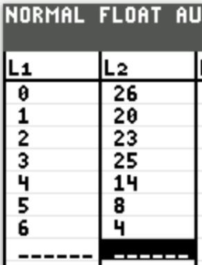
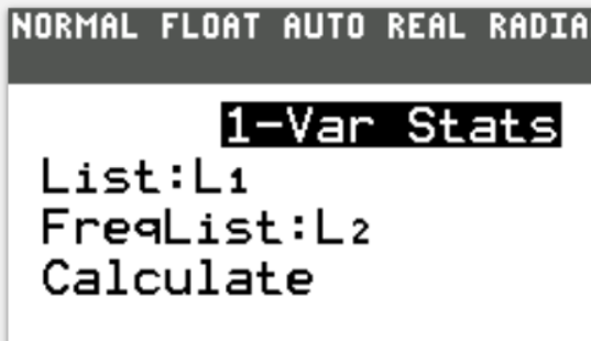
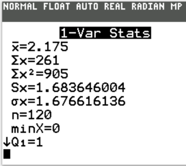
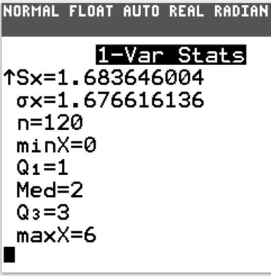
The table shows the numbers of letters delivered to the houses one day.
| Number of letters | 0 | 1 | 2 | 3 | 4 | 5 | 6 |
| Frequency | 26 | 20 | 23 | 25 | 14 | 8 | 4 |
Find
(i.) the mode
(ii.) the median
(iii.) the range
(iv.) the upper quartile
(v.) the mean.
(b.) This table shows the numbers of letters delivered to the houses in another street one day.
| Number of letters | 0 | 1 | 2 | 3 | 4 | 5 | 6 |
| Frequency | 18 | 31 | 27 | 18 | n | 12 | 5 |
The mean number of letters delivered in this street is 2.28.
Find the value of n.
| Number of letters, x | Frequency, F | $F * x$ |
|---|---|---|
| 0 | 26 | 0 |
| 1 | 20 | 20 |
| 2 | 23 | 46 |
| 3 | 25 | 75 |
| 4 | 14 | 56 |
| 5 | 8 | 40 |
| 6 | 4 | 24 |
| $\Sigma F = 120$ | $\Sigma Fx = 261$ |
$ (i.) \\[3ex] \text{Highest Frequency} = 26 \\[3ex] \text{Mode = number with the highest frequency} = 0 \\[3ex] (ii.) \\[3ex] \dfrac{\Sigma F}{2} = \dfrac{120}{2} = 60 \\[5ex] \underline{\text{From the top}} \\[3ex] 26 + 20 = 46 \\[3ex] 46 + 23 = 69...STOP...\text{Freqency of 60 is contained here} \\[3ex] \text{Median = data that contains frequency of 60} = 2 \\[3ex] (iii.) \\[3ex] \text{Range} = \text{maximum value} - \text{minimum value} \\[3ex] = 6 - 0 \\[3ex] = 6 \\[3ex] (iv.) \\[3ex] \dfrac{3}{4} * 120 = 90 \\[5ex] \text{Upper Quartile}, Q_3 = \dfrac{90th + 91st}{2} \\[5ex] 69 + 25 = 94...STOP...\text{the 90th and 91st value are contained here} \\[3ex] \text{90th and 91st value} = 3 \\[3ex] Q_3 = \dfrac{3 + 3}{2} \\[5ex] Q_3 = 3 \\[3ex] (v.) \\[3ex] \text{Mean}, \bar{x} = \dfrac{\Sigma Fx}{\Sigma F} \\[5ex] = \dfrac{261}{120} \\[5ex] = 2.175 \\[3ex] (b.) \\[3ex] $
| Number of letters, x | Frequency, F | $F * x$ |
|---|---|---|
| 0 | 18 | 0 |
| 1 | 31 | 31 |
| 2 | 27 | 54 |
| 3 | 18 | 54 |
| 4 | n | 4n |
| 5 | 12 | 60 |
| 6 | 5 | 30 |
| $\Sigma F = n + 111$ | $\Sigma Fx = 4n + 229$ |
$ \bar{x} = \dfrac{\Sigma Fx}{\Sigma F} \\[5ex] 2.28 = \dfrac{4n + 229}{n + 111} \\[5ex] 4n + 229 = 2.28(n + 111) \\[3ex] 4n + 229 = 2.28n + 253.08 \\[3ex] 4n - 2.28n = 253.08 - 229 \\[3ex] 1.72n = 24.08 \\[3ex] n = \dfrac{24.08}{1.72} \\[5ex] n = 14 $
Write down the probability that the die shows
(i.) a number less than 5
(ii.) an even number
(b.) Dilshan has two fair 6-sided dice each numbered from 1 to 6.
He throws both dice.
Find the probability that
(i.) both dice show a 6
(ii.) at least one die does not show a 6.
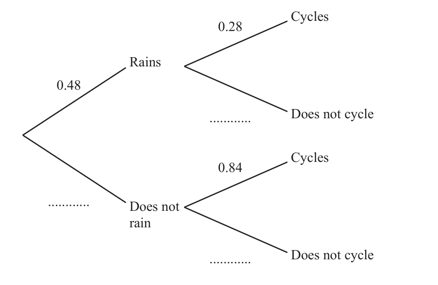
(c.) The probability that it rains on Wednesday is 0.48.
If it rains, the probability that Hannah cycles to work is 0.28.
If it does not rain, the probability that Hannah cycles to work is 0.84.
(i.) Complete this tree diagram.
(ii.) Find the probability that, on Wednesday, it does not rain and Hannah cycles.
$ (a.) \\[3ex] \text{Sample Space}, S = \{1, 2, 3, 4, 5, 6\} \\[3ex] n(S) = 6 \\[3ex] (i.) \\[3ex] \text{Event Space}, E = \{1, 2, 3, 4\} \\[3ex] n(E) = 4 \\[3ex] P(E) = \dfrac{n(E)}{n(S)} = \dfrac{4}{6} = \dfrac{2}{3} \\[5ex] (ii.) \\[3ex] \text{Event Space}, F = \{2, 4, 6\} \\[3ex] n(F) = 3 \\[3ex] P(F) = \dfrac{n(F)}{n(S)} = \dfrac{3}{6} = \dfrac{1}{2} \\[5ex] (b.) \\[3ex] \text{Sample Space for 1st Die}, S = \{1, 2, 3, 4, 5, 6\} \\[3ex] \text{Sample Space for 2nd Die}, S = \{1, 2, 3, 4, 5, 6\} \\[3ex] P(\text{6 on 1st die}) = \dfrac{1}{6} \\[5ex] P(\text{6 on 2nd die}) = \dfrac{1}{6} \\[5ex] P(\text{both dice show a 6}) \\[3ex] P(\text{6 on 1st die AND 6 on 2nd Die}) \\[3ex] = \dfrac{1}{6} * \dfrac{1}{6} ...\text{Multiplication Rule for Independent Events} \\[5ex] = \dfrac{1}{36} \\[5ex] $ (ii.) We can do this question using at least two approaches.
You may use any approach you prefer, however, I recommend the first approach.
$ \underline{\text{1st Approach: Complementary Event}} \\[3ex] \text{Event: K: at least one die does not show a 6} \\[3ex] \text{Complementary Event: K': both dice show a 6} \\[3ex] P(K) + P(K') = 1 ...\text{Complementary Rule} \\[3ex] P(K) + \dfrac{1}{36} = \dfrac{36}{36} \\[5ex] P(K) = \dfrac{36}{36} - \dfrac{1}{36} \\[5ex] P(K) = \dfrac{35}{36} \\[5ex] $ At least 1 means: 1 or more
In the context of the question: at least 1 means: 1 or 2
At least one die does not show a 6 implies
Case 1: 1st die does not show a 6 AND 2nd die shows a 6
OR
Case 2: 2nd die does not show a 6 AND 1st die shows a 6
OR
Case 3: 1st die does not show a 6 AND 2nd die does not show a 6
$ P(\text{any die shows a 6}) = \dfrac{1}{6} \\[5ex] P(\text{any die does not show a 6}) \\[3ex] = 1 - \dfrac{1}{6} ...\text{Complementary Rule} \\[5ex] = \dfrac{5}{6} \\[5ex] \underline{\text{2nd Approach: Long Approach: Possibilities}} \\[3ex] \underline{\text{Multiplication Rule for Independent Events}} \\[3ex] P(\text{Case 1}) = \dfrac{5}{6} * \dfrac{1}{6} = \dfrac{5}{36} \\[5ex] P(\text{Case 2}) = \dfrac{5}{6} * \dfrac{1}{6} = \dfrac{5}{36} \\[5ex] P(\text{Case 3}) = \dfrac{5}{6} * \dfrac{5}{6} = \dfrac{25}{36} \\[5ex] P(\text{at least one die does not show a 6}) \\[3ex] = P(\text{Case 1}) + P(\text{Case 2}) + P(\text{Case 3})...\text{Addition Rule for Independent Events} \\[3ex] = \dfrac{5}{36} + \dfrac{5}{36} + \dfrac{25}{36} \\[5ex] = \dfrac{35}{36} \\[5ex] (c.) \\[3ex] $ (i.) Let us use Complementary Rule to complete the tree diagram
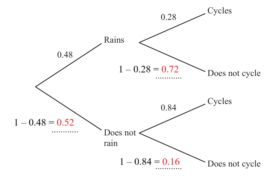
Let the event that:
It rains = R
It does not rain = R'
Hannah cycles = C
Hannah does not cycle = C'
$ (ii.) \\[3ex] P(R' \cap C) \\[3ex] = P(R') * P(C | R') ...\text{Multiplication Rule for Dependent Events} \\[3ex] = 0.52 * 0.84 \\[3ex] = 0.4368 $
Two cubes (dice) each have faces numbered 1, 2, 3, 4, 5 and 6.
In the game, a throw is rolling the two fair 6-sided dice and then adding the numbers on their top faces.
This total is the number of spaces to move on the board.
For example, if the numbers are 4 and 3, he moves 7 spaces.
(a.) Giving each of your answers as a fraction in its simplest form, find the probability that he moves
(i.) two spaces with his next throw,
(ii.) ten spaces with his next throw.
(b.) What is the most likely number of spaces that Kenwyn will move with his next throw?
Explain your answer.
(c.)
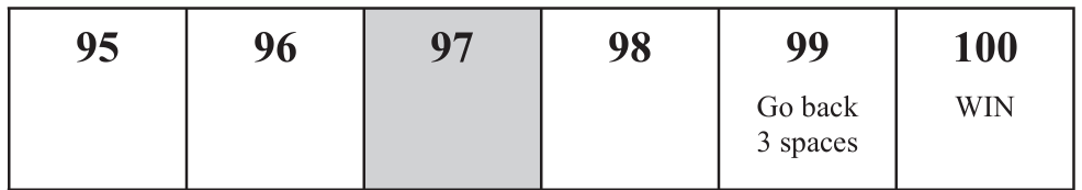
To win the game, he must move exactly to the 100th space.
Kenwyn is on the 97th space.
If his next throw takes him to 99, he has to move back to 96.
If his next throw takes him over 100, he stays on 97.
Find the probability that he reaches 100 in either of his next two throws.
There are at least two approaches that we can use to solve the question.
Having gone over the entire question, I prefer to use the Punnett Square.
If you want another approach besides the Punnett Square, please contact me.
|
1 Die → (+) 1 Die ↓ |
1 | 2 | 3 | 4 | 5 | 6 |
|---|---|---|---|---|---|---|
| 1 | 2 | 3 | 4 | 5 | 6 | 7 |
| 2 | 3 | 4 | 5 | 6 | 7 | 8 |
| 3 | 4 | 5 | 6 | 7 | 8 | 9 |
| 4 | 5 | 6 | 7 | 8 | 9 | 10 |
| 5 | 6 | 7 | 8 | 9 | 10 | 11 |
| 6 | 7 | 8 | 9 | 10 | 11 | 12 |
$ S = \text{Sample Space} \\[3ex] P = \text{Probability} \\[3ex] n = \text{cardinality of the event space} \\[3ex] n(S) = 6 * 6 = 36 \\[5ex] (a.)(i.) \\[3ex] \text{two spaces with his next throw} \\[3ex] = P(2) \\[3ex] = \dfrac{n(2)}{n(S)} \\[3ex] = \dfrac{1}{36} \\[5ex] (ii.) \\[3ex] \text{ten spaces with his next throw} \\[3ex] = P(10) \\[3ex] = \dfrac{n(10)}{n(S)} \\[3ex] = \dfrac{3}{36} \\[5ex] = \dfrac{1}{12} \\[5ex] (b.) \\[3ex] n(2) = 1 \\[3ex] n(3) = 2 \\[3ex] n(4) = 3 \\[3ex] n(5) = 4 \\[3ex] n(6) = 5 \\[3ex] n(7) = 6 \\[3ex] n(8) = 5 \\[3ex] n(9) = 4 \\[3ex] n(10) = 3 \\[3ex] n(11) = 2 \\[3ex] n(12) = 1 \\[3ex] $ The most likely number of spaces that Kenwyn will move with his next throw is 7 because it has the greatest sum of 6.
(c.) Find the probability that he reaches 100 in either of his next two throws.
Let E be the event that he reaches 100 in either of his next two throws.
either of his next two throws means in 1 throw OR in 2 throws.
Let us consider the possibilities for Kenwyn to move from the 97th space to the 100th space in 1 throw OR in 2 throws.
Case 1: He moves 3 spaces from 97th space to the 100th space
OR
*Case 2:*? He moves 1 space to the 98th space, and 2 spaces to the 100th space.
This case is not possible because a throw (which determines a move) is a sum of the top faces of two dice.
1 is not a sum in that regard.
Hence, this will not work.
OR
Case 2:1st: He moves 2 spaces to the 99th space.
This will take him back 3 spaces to the 96th space.
2nd: Then, he will move 4 spaces to the 100th space.
So, this case is: 2 spaces AND 4 spaces
The backward move is not considered a throw.
OR
Case 3:1st: He moves 4 through 12 spaces (4 or 5 or 6 or 7 or 8 or 9 or 10 or 11 or 12 spaces) over 100.
This makes him stay on the 97th space.
2nd: Then, he moves 3 spaces to the 100th space.
So, this case is: 4 – 12 spaces AND 3 spaces
$ \underline{\text{Case 1}} \\[3ex] P(3) = \dfrac{n(3)}{n(S)} = \dfrac{2}{36} = \dfrac{1}{18} \\[5ex] \underline{\text{Case 2}} \\[3ex] P(2) * P(4) ...\text{Multipication Rule for Independent Events} \\[3ex] = \dfrac{n(2)}{n(S)} * \dfrac{n(4)}{n(S)} \\[5ex] = \dfrac{1}{36} * \dfrac{3}{36} \\[5ex] = \dfrac{1}{36} * \dfrac{1}{12} \\[5ex] = \dfrac{1}{432} \\[5ex] \underline{\text{Case 3}} \\[3ex] P(4 \;—\; 12) * P(3) ...\text{Multipication Rule for Independent Events} \\[3ex] = \dfrac{n(4 \;—\; 12)}{n(S)} * \dfrac{n(3)}{n(S)} \\[5ex] = \dfrac{33}{36} * \dfrac{2}{36} \\[5ex] = \dfrac{11}{12} * \dfrac{1}{18} \\[5ex] = \dfrac{11}{216} \\[5ex] P(E) = \text{Case 1} + \text{case 2} + \text{Case 3}...\text{Addition Rule} \\[3ex] = \dfrac{1}{18} + \dfrac{1}{432} + \dfrac{11}{216} \\[5ex] = \dfrac{24 + 1 + 22}{432} \\[5ex] = \dfrac{47}{432} $


