Statistics and Probability
Welcome to Our Site
I greet you this day,
These are the solutions to questions on Statistics and Probability.
The TI-84 Plus CE shall be used for applicable questions.
If you find these resources valuable/helpful, please consider making a donation:
Cash App: $ExamsSuccess or
cash.app/ExamsSuccess
PayPal: @ExamsSuccess or
PayPal.me/ExamsSuccess
Google charges me for the hosting of this website and my other
educational websites. It does not host any of the websites for free.
Besides, I spend a lot of time to type the questions and the solutions well.
As you probably know, I provide clear explanations on the solutions.
Your donation is appreciated.
Comments, ideas, areas of improvement, questions, and constructive criticisms are welcome.
Feel free to contact me. Please be positive in your message.
I wish you the best.
Thank you.
-
Symbols and Meanings
- $X$ = dataset $X$
- $x = x-values$ OR data values
- $x_{mid}$ = class midpoint of $x-values$ = class midpoint of the data values
- $\Sigma$ (pronounced as uppercase Sigma) = $summation$
- $\Sigma x$ = summation of the $x-values$
- $f = frequency$
- $F = frequency$
- $\Sigma f$ = summation of the frequencies
- $\Sigma fx$ = summation of the product of the $x-values$ and their corresponding frequencies
- $(\Sigma x)^2$ = square of the summation of the $x-values$
- $\Sigma x^2$ = summation of the squared of the $x-values$
- $\bar{x}$ is sample mean of the $x-values$
- $\mu$ = population mean
- $n$ = sample size
- $N$ = population size
- $\tilde{x}$ = median
- $\widehat{x}$ = mode
- $AM$ = assumed mean
- $D$ = deviation from the assumed mean
- $x_{MR}$ = midrange
- $LCL$ = lower class limit
- $UCL$ = upper class limit
- $min$ = minimum data value
- $max$ = maximum data value
- $LCB_{med}$ = lower class boundary of the median class
- $CW$ = class width
- $f_{med}$ = frequency of the median class
- $CF_{bmed}$ = cumulative frequency of the class before the median class
- $LCB_{mod}$ = lower class boundary of the modal class
- $f_{mod}$ = frequency of the modal class
- $f_{bmod}$ = frequency of the class before the modal class
- $f_{amod}$ = frequency of the class after the modal class
- $R$ = range
- $s$ = sample standard deviation
- $s^2$ = sample variance
- $\sigma$ = population standard deviation
- $\sigma^2$ = population variance
- $CV$ = coefficient of variation
- $z = z-score$
- $Q_1$ = lower quartile or first quartile
- $P_{25}$ = 25th percentile or first quartile
- $Q_2$ = middle quartile or second quartile or median
- $P_{50}$ = 50th percentile or median
- $Q_3$ = upper quartile or third quartile
- $P_{75}$ = 75th percentile or third quartile
- $IQR$ = interquartile range
- $SIQR$ = semi-interquartile range
- $MQ$ = midquartile
- $LF$ = lower fence
- $UF$ = upper fence
- $TM$ = trimmed mean
- $\Pi$ (pronounced as uppercase Pi) = $product$
- $\Pi x$ = product of the $x-values$
- $GM$ = geometric mean
- CL = Confidence Level or Level of Confidence or Confidence Coefficient
- CI = Confidence Interval or Interval Estimate
- LCL = Lower confidence limit
- UCL = Upper confidence limit
- LCI = Length of confidence interval
- α = Level of Significance or Significance Level
- $z_{\dfrac{\alpha}{2}}$ = critical z value separating an area or probability of $\dfrac{\alpha}{2}$ in the right tail.
- $-z_{\dfrac{\alpha}{2}}$ = critical z value separating an area or probability of $\dfrac{\alpha}{2}$ in the left tail.
- $z_{\alpha}$ = critical z value separating an area or probability of α in the right tail.
- $-z_{\alpha}$ = critical z value separating an area or probability of α in the left tail.
- p̂ = sample proportion or estimated proportion of successes or point estimate of the population proportion
- q̂ = estimated proportion of failures
- p = population proportion
- SE = standard error
- SEest = estimated standard error
- x = number of individuals in the sample with the specified characteristic
- n = sample size or minimum sample size
- N = population size
- E = margin or error or maximum error of estimation or error bound
- $\bar{x}$ = sample mean or point estimate of the population mean
- μ = population mean
- s = sample standard deviation
- s² = sample variance
- σ = population standard deviation
- σ² = population variance
- $t_{\dfrac{\alpha}{2}}$ = critical t value separating an area or probability of $\dfrac{\alpha}{2}$ in the right tail (use for one-tailed tests)
- $t_{\alpha}$ = critical t value separating an area or probability of α in the right tail (use for two-tailed tests)
- df = degrees of freedom
- Χ² = Chi-Square distribution
- Χ²R = right-tailed (upper-tail) critical values of the Chi-Square distribution
- Χ²L = left-tailed (lower-tail) critical values of the Chi-Square distribution
- CI for Population Proportion in plus-minus notation = p̂ ± E
- CI for Population Proportion in interval notation = (p̂ − E, p̂ + E)
- CI for Population Proportion in trilinear inequality = p̂ − E < p < p̂ + E
- CI for Population Mean in plus-minus notation = x̄ ± E
- CI for Population Mean in interval notation = (x̄ − E, x̄ + E)
- CI for Population Mean in trilinear inequality = x̄ − E < p < x̄ + E
Grouped Data
$
\underline{\text{Class Size or Class Width}} \\[3ex]
(1.)\;\; Class\:\:Width = \dfrac{Maximum - Minimum}{Number\:\:of\:\:classes} \\[5ex]
(2.)\;\; Class\:\:Width = LCI\:\:of\:\:2nd\:\:Class - LCI\:\:of\:\:1st\:\:Class \\[3ex]
(3.)\;\; Class\:\:Width = UCI\:\:of\:\:2nd\:\:Class - UCI\:\:of\:\:1st\:\:Class \\[3ex]
(4.)\;\; Class\:\:Width = UCB\:\:of\:\:a\:\:class - LCB\:\:of\:\:the\:\:same\:\:class \\[3ex]
(5.)\;\; Class\:\:Width = LCB\:\:of\:\:a\:\:Class - LCB\:\:of\:\:previous\:\:class \\[5ex]
\underline{\text{Frequency Density}} \\[3ex]
(6.)\;\; \text{Frequency Density} = \dfrac{\text{Frequency}}{\text{Class Width}} \\[7ex]
\underline{\text{Class Midpoints or Class Marks}} \\[3ex]
(7.)\;\; Class\:\:Width = LCB\:\:of\:\:a\:\:Class - LCB\:\:of\:\:previous\:\:class \\[5ex]
\underline{\text{Class Boundaries}} \\[3ex]
(8.)\;\; Lower\:\:Class\:\:Boundary\:\:of\:\:a\:\:class = \dfrac{LCI\:\:of\:\:that\:\:class +
UCI\:\:of\:\:previous/preceding\:\:class}{2} \\[5ex]
(9.)\;\; Upper\:\:Class\:\:Boundary\:\:of\:\:a\:\:class = \dfrac{UCI\:\:of\:\:that\:\:class +
LCI\:\:of\:\:next/succeeding\:\:class}{2} \\[5ex]
$
(10.) Shortcut for Class Boundaries
If the class intervals are integers:
Lower Class Boundary = Lower Class Interval − 0.5
Upper Class Boundary = Upper Class Interval + 0.5
If the class intervals are decimals in one decimal place:
Lower Class Boundary = Lower Class Interval − 0.05
Upper Class Boundary = Upper Class Interval + 0.05
If the class intervals are decimals in two decimal places:
Lower Class Boundary = Lower Class Interval − 0.005
Upper Class Boundary = Upper Class Interval + 0.005
...and so on and so forth.
$
\underline{\text{Relative Frequency}} \\[3ex]
(11.)\;\; RF\:\:of\:\:a\:\:class = \dfrac{Frequency\:\:of\:\:that\:\:class}{\Sigma Frequency} \\[7ex]
\underline{\text{Cumulative Frequency}} \\[3ex]
(12.)\;\; CF\:\:of\:\:1st\:\:Class = Frequency\:\:of\:\:1st\:\:Class \\[3ex]
CF\:\:of\:\:2nd\:\:Class = Frequency\:\:of\:\:1st\:\:Class + Frequency\:\:of\:\:2nd\:\:Class \\[3ex]
CF\:\:of\:\:3rd\:\:Class = Frequency\:\:of\:\:1st\:\:Class + Frequency\:\:of\:\:2nd\:\:Class +
Frequency\:\:of\:\:3rd\:\:Class \\[3ex]
CF = CF\:\:of\:\:Last\:\:Class = \Sigma Frequency
$
Measures of Center: Raw Data and Ungrouped Data
$ \underline{Sample\:\:Mean} \\[3ex] (1.)\:\: \bar{x} = \dfrac{\Sigma x}{n} \\[5ex] (2.)\:\: n = \Sigma f \\[3ex] (3.)\:\: \bar{x} = \dfrac{\Sigma fx}{\Sigma f} \\[5ex] \underline{Given\:\:an\:\:Assumed\:\:Mean} \\[3ex] (4.)\:\: D = x - AM \\[3ex] (5.)\:\: \bar{x} = AM + \dfrac{\Sigma D}{n} \\[5ex] (6.)\:\: \bar{x} = AM + \dfrac{\Sigma fD}{\Sigma f} \\[7ex] \underline{Population\:\:Mean} \\[3ex] (7.)\:\: \mu = \dfrac{\Sigma x}{N} \\[5ex] (8.)\:\: N = \Sigma f \\[3ex] \underline{Given\:\:an\:\:Assumed\:\:Mean} \\[3ex] (9.)\:\: D = x - AM \\[3ex] (10.)\:\: \mu = AM + \dfrac{\Sigma D}{N} \\[5ex] (11.)\:\: \mu = AM + \dfrac{\Sigma fD}{\Sigma f} \\[7ex] \underline{Median} \\[3ex] (12.)\:\: \tilde{x} = \left(\dfrac{\Sigma f + 1}{2}\right)th \:\:for\:\:sorted\:\:odd\:\:sample\:\:size \\[5ex] (13.)\:\: \tilde{x} = \left(\dfrac{\Sigma f}{2}\right)th \:\:for\:\:sorted\:\:even\:\:sample\:\:size \\[7ex] \underline{Mode} \\[3ex] (14.)\:\: Mode = x-value(s) \:\;with\:\:highest\:\:frequency \\[5ex] \underline{Midrange} \\[3ex] (15.)\:\: x_{MR} = \dfrac{min + max}{2} \\[5ex] \underline{Geometric\;\;Mean} \\[3ex] (16.)\;\; GM = \sqrt[n]{\prod\limits_{x=1}^n x} $
Measures of Center: Grouped Data
$ \underline{Class\:\:Midpoint} \\[3ex] (1.)\:\: x_{mid} = \dfrac{LCL + UCL}{2} \\[7ex] Equal\:\:Class\:\:Intervals\:(Same\:\:Class\:\:Size) \\[3ex] \underline{Mean} \\[3ex] (2.)\:\: \bar{x} = \dfrac{\Sigma fx_{mid}}{\Sigma f} \\[7ex] Equal\:\:Class\:\:Intervals\:(Same\:\:Class\:\:Size) \\[3ex] \underline{Given\:\:an\:\:Assumed\:\:Mean} \\[3ex] (3.)\:\: D = x_{mid} - AM \\[3ex] (4.)\:\: \bar{x} = AM + \dfrac{\Sigma fD}{\Sigma f} \\[7ex] \underline{Median} \\[3ex] (5.)\:\: \tilde{x} = LCB_{med} + \dfrac{CW}{f_{med}} * \left[\left(\dfrac{\Sigma f}{2}\right) - CF_{bmed}\right] \\[7ex] \underline{Mode} \\[3ex] (6.)\:\: \widehat{x} = LCB_{mod} + CW * \left[\dfrac{f_{mod} - f_{bmod}}{(f_{mod} - f_{bmod}) + (f_{mod} - f_{amod})}\right] $
Measures of Spread: Raw Data and Ungrouped Data
$ \underline{Range} \\[3ex] (1.)\:\: Range = max - min \\[3ex] \underline{Using\;\;Assumed\;\;Mean} \\[3ex] (2.)\;\; D = x - AM \\[5ex] \underline{Sample\:\:Variance} \\[3ex] \color{red}{First\:\:Formula} \\[3ex] (3.)\:\: s^2 = \dfrac{\Sigma(x - \bar{x})^2}{n - 1} \\[5ex] (4.)\:\: s^2 = \dfrac{\Sigma f(x - \bar{x})^2}{\Sigma f - 1} \\[5ex] \color{red}{Second\:\:Formula} \\[3ex] (5.)\:\: s^2 = \dfrac{n(\Sigma x^2) - (\Sigma x)^2}{n(n - 1)} \\[5ex] (6.)\:\: s^2 = \dfrac{\Sigma f(\Sigma fx^2) - (\Sigma fx)^2}{\Sigma f(\Sigma f - 1)} \\[7ex] \underline{Using\;\;Assumed\;\;Mean} \\[3ex] (7.)\;\; s^2 = \dfrac{\Sigma D^2}{n - 1} - \left(\dfrac{\Sigma D}{n - 1}\right)^2 \\[7ex] (8.)\;\; s^2 = \dfrac{\Sigma fD^2}{\Sigma f - 1} - \left(\dfrac{\Sigma fD}{\Sigma f - 1}\right)^2 \\[10ex] \underline{Population\:\:Variance} \\[3ex] \color{red}{First\:\:Formula} \\[3ex] (9.)\:\: \sigma^2 = \dfrac{\Sigma(x - \mu)^2}{N} \\[5ex] (10.)\:\: \sigma^2 = \dfrac{\Sigma f(x - \mu)^2}{\Sigma f} \\[5ex] \color{red}{Second\:\:Formula} \\[3ex] (11.)\:\: \sigma^2 = \dfrac{N(\Sigma x^2) - (\Sigma x)^2}{N^2} \\[5ex] (12.)\:\: \sigma^2 = \dfrac{\Sigma f(\Sigma fx^2) - (\Sigma fx)^2}{(\Sigma f)^2} \\[7ex] \underline{Using\;\;Assumed\;\;Mean} \\[3ex] (13.)\;\; \sigma^2 = \dfrac{\Sigma D^2}{N} - \left(\dfrac{\Sigma D}{N}\right)^2 \\[7ex] (14.)\;\; \sigma^2 = \dfrac{\Sigma fD^2}{\Sigma f} - \left(\dfrac{\Sigma fD}{\Sigma f}\right)^2 \\[10ex] \underline{Sample\:\:Standard\:\:Deviation} \\[3ex] \color{red}{First\:\:Formula} \\[3ex] (15.)\:\: s = \sqrt{\dfrac{\Sigma(x - \bar{x})^2}{n - 1}} \\[5ex] (16.)\:\: s = \sqrt{\dfrac{\Sigma f(x - \bar{x})^2}{\Sigma f - 1}} \\[5ex] \color{red}{Second\:\:Formula} \\[3ex] (17.)\:\: s = \sqrt{\dfrac{n(\Sigma x^2) - (\Sigma x)^2}{n(n - 1)}} \\[5ex] (18.)\:\: s = \sqrt{\dfrac{\Sigma f(\Sigma fx^2) - (\Sigma fx)^2}{\Sigma f(\Sigma f - 1)}} \\[7ex] \underline{Using\;\;Assumed\;\;Mean} \\[3ex] (19.)\;\; s = \sqrt{\dfrac{\Sigma D^2}{n - 1} - \left(\dfrac{\Sigma D}{n - 1}\right)^2} \\[7ex] (20.)\;\; s = \sqrt{\dfrac{\Sigma fD^2}{\Sigma f - 1} - \left(\dfrac{\Sigma fD}{\Sigma f - 1}\right)^2} \\[10ex] \underline{Population\:\:Standard\:\:Deviation} \\[3ex] \color{red}{First\:\:Formula} \\[3ex] (21.)\:\: \sigma = \sqrt{\dfrac{\Sigma(x - \mu)^2}{N}} \\[5ex] (22.)\:\: \sigma = \sqrt{\dfrac{\Sigma f(x - \mu)^2}{\Sigma f}} \\[5ex] \color{red}{Second\:\:Formula} \\[3ex] (23.)\:\: \sigma = \dfrac{\sqrt{N(\Sigma x^2) - (\Sigma x)^2}}{N} \\[5ex] (24.)\:\: \sigma = \dfrac{\sqrt{\Sigma f(\Sigma fx^2) - (\Sigma fx)^2}}{\Sigma f} \\[7ex] \underline{Using\;\;Assumed\;\;Mean} \\[3ex] (25.)\;\; \sigma = \sqrt{\dfrac{\Sigma D^2}{N} - \left(\dfrac{\Sigma D}{N}\right)^2} \\[7ex] (26.)\;\; \sigma = \sqrt{\dfrac{\Sigma fD^2}{\Sigma f} - \left(\dfrac{\Sigma fD}{\Sigma f}\right)^2} \\[10ex] \underline{Range\:\:Rule\:\:of\:\:Thumb} \\[3ex] Approximate\:\:Value\:\:of\:\:Calculating\:\:Standard\:\:Deviation \\[3ex] (27.)\:\: s = \dfrac{Range}{4} = \dfrac{max - min}{4} \\[7ex] \underline{Interquartile\:\:Range} \\[3ex] (28.)\:\: IQR = Q_3 - Q_1 \\[5ex] \underline{Coefficient\:\:of\:\:Variation\:\:for\:\:Sample} \\[3ex] (29.)\:\: CV = \dfrac{s}{x} * 100 ...in\:\:\% \\[7ex] \underline{Coefficient\:\:of\:\:Variation\:\:for\:\:Population} \\[3ex] (30.)\:\: CV = \dfrac{\sigma}{x} * 100 ...in\:\:\% \\[7ex] \underline{Mean\:\:Absolute\:\:Deviation} \\[3ex] (31.)\:\: MAD = \dfrac{\Sigma |x - \bar{x}|}{n} \\[5ex] \underline{Mean\:\:Absolute\:\:Deviation} \\[3ex] (32.)\:\: MAD = \dfrac{\Sigma f|x - \bar{x}|}{\Sigma f} \\[5ex] $
Measures of Spread: Grouped Data
$ \underline{Class\:\:Midpoint} \\[3ex] (1.)\:\: x_{mid} = \dfrac{LCL + UCL}{2} \\[5ex] \underline{Using\;\;Assumed\;\;Mean} \\[3ex] (2.)\;\; D = x_{mid} - AM \\[5ex] \underline{Sample\:\:Variance} \\[3ex] \color{red}{First\:\:Formula} \\[3ex] (3.)\:\: s^2 = \dfrac{\Sigma f(x_{mid} - \bar{x})^2}{\Sigma f - 1} \\[5ex] \color{red}{Second\:\:Formula} \\[3ex] (4.)\:\: s^2 = \dfrac{\Sigma f(\Sigma fx_{mid}^2) - (\Sigma fx_{mid})^2}{\Sigma f(\Sigma f - 1)} \\[5ex] \underline{Using\;\;Assumed\;\;Mean} \\[3ex] (5.)\;\; s^2 = \dfrac{\Sigma D^2}{n - 1} - \left(\dfrac{\Sigma D}{n - 1}\right)^2 \\[7ex] (6.)\;\; s^2 = \dfrac{\Sigma fD^2}{\Sigma f - 1} - \left(\dfrac{\Sigma fD}{\Sigma f - 1}\right)^2 \\[10ex] \underline{Sample\:\:Standard\:\:Deviation} \\[3ex] \color{red}{First\:\:Formula} \\[3ex] (7.)\:\: s = \sqrt{\dfrac{\Sigma f(x_{mid} - \bar{x})^2}{\Sigma f - 1}} \\[5ex] \color{red}{Second\:\:Formula} \\[3ex] (8.)\:\: s = \sqrt{\dfrac{\Sigma f(\Sigma fx_{mid}^2) - (\Sigma fx_{mid})^2}{\Sigma f(\Sigma f - 1)}} \\[5ex] \underline{Using\;\;Assumed\;\;Mean} \\[3ex] (9.)\;\; s = \sqrt{\dfrac{\Sigma D^2}{n} - \left(\dfrac{\Sigma D}{n - 1}\right)^2} \\[7ex] (10.)\;\; s = \sqrt{\dfrac{\Sigma fD^2}{\Sigma f - 1} - \left(\dfrac{\Sigma fD}{\Sigma f - 1}\right)^2} \\[10ex] \underline{Population\:\:Variance} \\[3ex] \color{red}{First\:\:Formula} \\[3ex] (11.)\:\: \sigma^2 = \dfrac{\Sigma f(x_{mid} - \bar{x})^2}{\Sigma f} \\[5ex] \color{red}{Second\:\:Formula} \\[3ex] (12.)\:\: \sigma^2 = \dfrac{\Sigma f(\Sigma fx_{mid}^2) - (\Sigma fx_{mid})^2}{\Sigma f(\Sigma f)} \\[5ex] \underline{Using\;\;Assumed\;\;Mean} \\[3ex] (13.)\;\; \sigma^2 = \dfrac{\Sigma D^2}{N} - \left(\dfrac{\Sigma D}{N}\right)^2 \\[7ex] (14.)\;\; \sigma^2 = \dfrac{\Sigma fD^2}{\Sigma f} - \left(\dfrac{\Sigma fD}{\Sigma f}\right)^2 \\[10ex] \underline{Population\:\:Standard\:\:Deviation} \\[3ex] \color{red}{First\:\:Formula} \\[3ex] (15.)\:\: \sigma = \sqrt{\dfrac{\Sigma f(x_{mid} - \bar{x})^2}{\Sigma f}} \\[5ex] \color{red}{Second\:\:Formula} \\[3ex] (16.)\:\: \sigma = \sqrt{\dfrac{\Sigma f(\Sigma fx_{mid}^2) - (\Sigma fx_{mid})^2}{\Sigma f(\Sigma f)}} \\[5ex] \underline{Using\;\;Assumed\;\;Mean} \\[3ex] (17.)\;\; \sigma = \sqrt{\dfrac{\Sigma D^2}{N} - \left(\dfrac{\Sigma D}{N}\right)^2} \\[7ex] (18.)\;\; \sigma = \sqrt{\dfrac{\Sigma fD^2}{\Sigma f} - \left(\dfrac{\Sigma fD}{\Sigma f}\right)^2} \\[10ex] $
Measures of Position
A data value is usual if $-2.00 \le z-score \le 2.00$
A data value is unusual if $z-score \lt -2.00$ OR $z-score \gt 2.00$
$
\underline{Sample} \\[3ex]
Minimum\:\:usual\:\:data\:\:value = \bar{x} - 2s \\[3ex]
Maximum\:\:usual\:\:data\:\:value = \bar{x} + 2s \\[5ex]
\underline{Population} \\[3ex]
Minimum\:\:usual\:\:data\:\:value = \mu - 2\sigma \\[3ex]
Maximum\:\:usual\:\:data\:\:value = \mu + 2\sigma \\[5ex]
\underline{z\:\:score\:\:for\:\:Sample} \\[3ex]
(1.)\:\: z = \dfrac{x - \bar{x}}{s} \\[7ex]
\underline{z\:\:score\:\:for\:\:Population} \\[3ex]
(2.)\:\: z = \dfrac{x - \mu}{\sigma} \\[7ex]
\underline{Quantiles(Percentiles,\:Deciles,\:Quintiles,\:and\:Quartiles)} \\[3ex]
\color{red}{Convert\:\:a\:\:Data\:\:value\:\:to\:\:a\:\:Quantile} \\[3ex]
x\:\:and\:\:y\:\:are\:\:two\:\:different\:\:variables \\[3ex]
(3.)\:\: Percentile\:\:of\:\:x =
\dfrac{number\:\:of\:\:values\:\:less\:\:than\:\:x}{total\:\:number\:\:of\:\:values} * 100 = yth\:\:Percentile
\\[5ex]
(4.)\:\: Decile\:\:of\:\:x =
\dfrac{number\:\:of\:\:values\:\:less\:\:than\:\:x}{total\:\:number\:\:of\:\:values} * 10 = yth\:\:Decile
\\[5ex]
(5.)\:\: Quintile\:\:of\:\:x =
\dfrac{number\:\:of\:\:values\:\:less\:\:than\:\:x}{total\:\:number\:\:of\:\:values} * 5 = yth\:\:Quintile
\\[5ex]
(6.)\:\: Quartile\:\:of\:\:x =
\dfrac{number\:\:of\:\:values\:\:less\:\:than\:\:x}{total\:\:number\:\:of\:\:values} * 4 = yth\:\:Quartile
\\[7ex]
\color{red}{Convert\:\:a\:\:Quantile\:\:to\:\:a\:\:Data\:\:Value} \\[3ex]
Calculate\:\:the\:\:xth\:\:position\:\:of\:\:the\:\:yth\:\:Quantile \\[3ex]
(7.)\:\: xth\:\:position = \dfrac{yth\:\:Percentile}{100} * total\:\:number\:\:of\:\:values \\[5ex]
(8.)\:\: xth\:\:position = \dfrac{yth\:\:Decile}{10} * total\:\:number\:\:of\:\:values \\[5ex]
(9.)\:\: xth\:\:position = \dfrac{yth\:\:Quintile}{5} * total\:\:number\:\:of\:\:values \\[5ex]
(10.)\:\: xth\:\:position = \dfrac{yth\:\:Quartile}{4} * total\:\:number\:\:of\:\:values \\[7ex]
$
| If the $xth$ position | then, |
|---|---|
| is an integer |
$xth\:\:position = \dfrac{xth\:\:position + (x + 1)th\:\;position}{2}$ In other words, find the value of the $xth$ position; find the value of the next position; and determine the mean of the two values. |
| is not an integer | $xth$ position is rounded up |
$ \underline{The\:\:Five-Number\:\:Summary\:\:of\:\:Data} \\[3ex] (11.)\:\: Minimum\:(min) \\[3ex] (12.)\:\: Lower\:\:Quartile\:(Q_1) \\[3ex] (13.)\:\: Median\:\:or\:\:Middle\:\:Quartile\:(Q_2) \\[3ex] (14.)\:\: Upper\:\:Quartile\:(Q_3) \\[3ex] (15.)\:\: Maximum\:(Max) \\[5ex] \underline{Other\:\:Statistics\:\:from\:\:Quantiles} \\[3ex] (16.)\:\: IQR = Q_3 - Q_1 \\[3ex] (17.)\:\: SIQR = \dfrac{IQR}{2} = \dfrac{Q_3 - Q_1}{2} \\[5ex] (18.)\:\: MQ = \dfrac{Q_3 + Q_1}{2} \\[5ex] (19.)\:\: Upper\:\:Quartile\:(Q_3) \\[3ex] (20.)\:\: LF = Q_1 - 1.5(IQR) \\[3ex] (21.)\:\: UF = Q_3 + 1.5(IQR) $
Probability
Given any two events say A and B
$
P(E) = \dfrac{n(E)}{n(S)} \\[5ex]
\underline{\text{Addition Rule}} \\[3ex]
\dfrac{n(A \cup B)}{n(S)} = \dfrac{n(A)}{n(S)} + \dfrac{n(B)}{n(S)} - \dfrac{n(A \cap B)}{n(S)} \\[5ex]
P(A \cup B) = P(A) + P(B) - P(A \cap B) \\[3ex]
P(A\:\:\:OR\:\:\:B) = P(A) + P(B) - P(A\:\:\:AND\:\:\:B) \\[5ex]
$
For Independent Events
$
P(B|A) = P(B) \\[3ex]
\rightarrow P(A\:\:\:OR\:\:\:B) = P(A) + P(B) - [P(A) * P(B)] \\[5ex]
$
For Dependent Events
$
P(B|A) = P(B|A) \\[3ex]
\rightarrow P(A\:\:\:OR\:\:\:B) = P(A) + P(B) - [P(A) * P(B|A)] \\[5ex]
$
For Mutually Exclusive Events (Disjoint Events)
$
P(A \cap B) = 0 \\[3ex]
P(A\:\:\:OR\:\:\:B) = P(A) + P(B) - 0 \\[3ex]
\rightarrow P(A\:\:\:OR\:\:\:B) = P(A) + P(B) \\[5ex]
$
$
\underline{\text{Multiplication Rule}} \\[3ex]
P(A\:\:\:AND\:\:\:B) = P(A) * P(B|A) \\[3ex]
P(A \cap B) = P(A) * P(B|A) \\[3ex]
P(A\:\:\:AND\:\:\:B) = P(A \cap B) \\[5ex]
$
$P(B|A)$ is read as: the probability of event $B$ given event $A$
For Independent Events
$
P(B|A) = P(B) \\[3ex]
\rightarrow P(A\:\:\:AND\:\:\:B) = P(A) * P(B) \\[5ex]
$
For Dependent Events
$
P(B|A) = P(B|A) \\[3ex]
\rightarrow P(A\:\:\:AND\:\:\:B) = P(A) * P(B|A) \\[5ex]
$
The complement of Event $A$ is $A'$
$
\underline{Complementary\;\;Rule} \\[3ex]
P(A) + P(A') = 1 \\[3ex]
\rightarrow P(A') = 1 - P(A) \\[5ex]
$
Other Formulas
$
(1.)\;\; P(A) = P(A \cap B') + P(A \cap B)
$
Probability Distributions
$
\boldsymbol{Probability\;\;Distribution} \\[3ex]
(1.)\;\;\mu = \Sigma[x * P(x)] \\[3ex]
(2.)\;\;E = \Sigma[x * P(x)] \\[3ex]
(3.)\;\; \sigma = \sqrt{\Sigma[x^2 * P(x)] - \mu^2} \\[7ex]
\boldsymbol{Combinatorics} \\[3ex]
(1.)\:\: 0! = 1 \\[3ex]
(2.)\:\: n! = n * (n - 1) * (n - 2) * (n - 3) * ... * 1 \\[3ex]
(3.)\;\; n! = n * (n - 1)! \\[3ex]
(4.)\;\; n! = (n - 1) * (n - 2)!...among\;\;others \\[3ex]
(5.)\:\: C(n, x) = \dfrac{n!}{(n - x)!x!} \\[5ex]
(6.)\;\; C(n, x) = C(n, n - x) \\[7ex]
\boldsymbol{Binomial\;\;Distribution} \\[3ex]
(1.)\;\; p + q = 1 \\[3ex]
(2.)\;\; \mu = n * p \\[3ex]
(3.)\;\; \sigma = \sqrt{n * p * q} \\[4ex]
(4.)\;\; P(x) = C(n, x) * p^x * q^{n - x}...\text{Depends on the context of the question} \\[5ex]
where \\[3ex]
x = \text{number of successes/failures} \\[3ex]
n = \text{number of trials} = 12 \\[3ex]
C(n, x) = \text{Binomial coefficient} \\[3ex]
P(x) = \text{Probability of the number of successes/failures} \\[3ex]
p = \text{probability of success} = 70\% = 0.7 \\[3ex]
q = \text{probability of failure} = 1 - 0.7 = 0.3 \\[5ex]
\boldsymbol{Poisson\;\;Distribution} \\[3ex]
(1.)\;\;P(x) = \dfrac{\mu^x * e^{-\mu}}{x!} \\[5ex]
(2.)\;\; \mu = \sigma^2 \\[7ex]
\boldsymbol{Normal\;\;Distribution} \\[3ex]
(1.)\;\; z = \dfrac{x - \bar{x}}{s} \\[5ex]
(2.)\;\; x = \bar{x} + zs \\[3ex]
(3.)\;\; z = \dfrac{x - \mu}{\sigma} \\[5ex]
(4.)\;\; x = \mu + z\sigma \\[3ex]
(5.)\;\;\text{Probability Density Function},\;\;P(x) =
\dfrac{1}{\sigma\sqrt{2\pi}}e^{{-\dfrac{1}{2}}\left(\dfrac{x - \mu}{\sigma}\right)^2} \\[7ex]
$
Empirical Rule (68 - 95 - 99.7 percent Rule)
(Applies only to Normal Distribution)
(a.) 68% of the data lie within (below and above) 1 standard deviation of the mean
(b.) 95% of the data lie within (below and above) 2 standard deviations of the mean
(c.) 99.7% of the data lie within (below and above) 3 standard deviations of the mean
Pafnuty Chebyshev's Theorem
(Applies to any distribution)
At least $\left(1 - \dfrac{1}{k^2}\right) * 100$ % of the data lie within $k$ standard deviations of the mean
implies
At least $\left(1 - \dfrac{1}{k^2}\right) * 100$ % of the data lie within $\mu - k\sigma$ and $\mu + k\sigma$
Range Rule of Thumb
Minimum Usual Value = μ - 2σ
Maximum Usual Value = μ + 2σ
A data value is unusual if it is less than the minimum usual value or greater than the
maximum usual value
z-score Boundary
A data value is usual if −2.00 ≤ z-score ≤ 2.00
A data value is unusual if z-score < −2.00 or if z-score > 2.00
Critical z-values
| Significance Level, α | Confidence Level, CL | critical z value separating an area or probability of $\dfrac{\alpha}{2}$ in the right tail, $z_{\dfrac{\alpha}{2}}$ |
|---|---|---|
| 1% (0.01) | 99% (0.99) | 2.575829306443923 ≈ 2.576 |
| 5% (0.05) | 95% (0.95) | 1.9599639861189817 ≈ 1.96 |
| 10% (0.1) | 90% (0.9) | 1.6448536251332162 ≈ 1.64 |
Inferential Statistics: Population Proportion
$ (1.)\;\; \alpha = 1 - CL ...\text{in decimal} \\[5ex] (2.)\:\: \hat{p} = \dfrac{x}{n} \\[5ex] (3.)\:\: \hat{p} + \hat{q} = 1 \\[5ex] (4.)\;\; \hat{p} = \dfrac{UCL + LCL}{2} \\[5ex] (5.)\;\; E = \dfrac{UCL - LCL}{2} \\[5ex] (6.)\:\: E = z_{\dfrac{\alpha}{2}} * \sqrt{\dfrac{\hat{p} * \hat{q}}{n}} \\[7ex] (7.)\;\; n = \dfrac{0.25 * \left(z_{\dfrac{\alpha}{2}}\right)^2}{E^2} \\[7ex] (8.)\;\; n = \dfrac{\left(z_{\dfrac{\alpha}{2}}\right)^2 * \hat{p} * \hat{q}}{E^2} $
Inferential Statistics: Population Mean
$ (1.)\;\; \alpha = 1 - CL ...in\;\;decimal \\[5ex] (2.)\;\; LCI = UCL - LCL \\[5ex] (3.)\:\: \bar{x} = \dfrac{\Sigma x}{n} \\[7ex] (4.)\:\: \bar{x} = \dfrac{UCL + LCL}{2} \\[7ex] (5.)\;\; E = \dfrac{UCL - LCL}{2} \\[7ex] (6.)\;\; LCI = 2E \\[5ex] (7.)\;\; SE = \dfrac{\sigma}{\sqrt{n}} \\[7ex] (8.)\:\: E = \dfrac{\sigma * z_{\dfrac{\alpha}{2}}}{\sqrt{n}} \\[10ex] (9.)\;\; E = \dfrac{s * t_{\dfrac{\alpha}{2}}}{\sqrt{n}} \\[10ex] (10.)\;\; n = \left(\dfrac{\sigma * z_{\dfrac{\alpha}{2}}}{E}\right)^2 \\[10ex] (11.)\;\; n = \left(\dfrac{s * t_{\dfrac{\alpha}{2}}}{E}\right)^2 \\[10ex] $
On average, 8 children out of 10 can jump a height of more than 127 cm, and 1 child out of 3 can jump a height of more than 135 cm.
(a.) Determine the mean and standard deviation of the heights the children can jump.
(b.) Determine the probability that a randomly chosen child will not be able to jump a height of 145 cm.
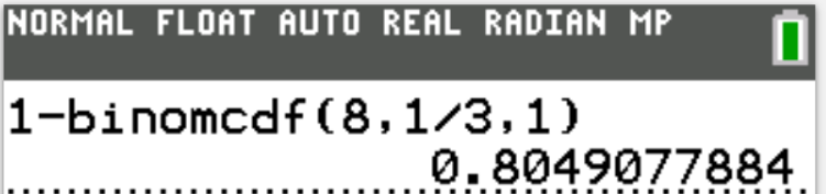
(c.) Determine the probability that, of 8 randomly chosen children, at least 2 will be able to jump a height of more than 135 cm.
Use only tables in your work.
You may verify with a calculator.
Let X be the event that a child of a particular age can jump more than a certain height
(a.) and (b.) deals with Normal Probability Distribution
(c.) deals with Binomial Probability Distribution
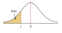
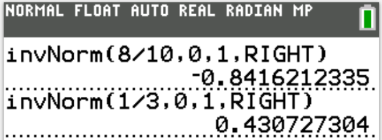
$ (a.) \\[3ex] P(X \gt 127) = \dfrac{8}{10} = 0.8 \\[3ex] P(X \lt 127) = 1 - 0.8 = 0.2 ...\text{Because of Standard Normal Table Left-Shaded Area} \\[3ex] \text{Convert to a z-score }: P(z \lt what) = 0.2 \\[3ex] $
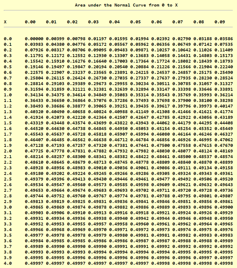
| z-scores | Areas |
|---|---|
| −0.84 | 0.20045 |
| z | 0.2 |
| −0.85 | 0.19766 |
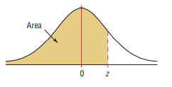
$ \dfrac{z - -0.85}{-0.84 - -0.85} = \dfrac{0.2 - 0.19766}{0.20045 - 0.19766} \\[5ex] \dfrac{z + 0.85}{0.01} = \dfrac{0.00234}{0.00279} \\[5ex] z = 0.01(0.8387096774) - 0.85 \\[3ex] z = -0.8416129032 \\[3ex] z = \dfrac{x - \mu}{\sigma} \\[5ex] \dfrac{127 - \mu}{\sigma} = -0.8416129032 \\[5ex] 127 - \mu = -0.8416129032\sigma...eqn.(1) \\[5ex] P(X \gt 135) = \dfrac{1}{3} = 0.3\bar{3} \\[3ex] P(X \lt 135) = 1 - 0.3\bar{3} = 0.66667 ...\text{Because of Standard Normal Table Left-Shaded Area} \\[3ex] \text{Convert to a z-score }: P(z \lt what) = 0.66667 \\[3ex] $
| z-scores | Areas |
|---|---|
| 0.44 | 0.67003 |
| z | 0.66667 |
| 0.43 | 0.66640 |
$ \dfrac{z - 0.43}{0.44 - 0.43} = \dfrac{0.66667 - 0.66640}{0.67003 - 0.66640} \\[5ex] \dfrac{z - 0.43}{0.01} = \dfrac{0.00027}{0.00363} \\[5ex] z = 0.01(0.0743801653) + 0.43 \\[3ex] z = 0.4307438017 \\[3ex] z = \dfrac{x - \mu}{\sigma} \\[5ex] \dfrac{135 - \mu}{\sigma} = 0.4307438017 \\[5ex] 135 - \mu = 0.4307438017\sigma...eqn.(2) \\[5ex] eqn.(2) - eqn.(1) \rightarrow \\[3ex] 135 - \mu - (127 - \mu) = 0.4307438017\sigma - -0.8416129032\sigma \\[3ex] 135 - \mu - 127 + \mu = 1.272356705\sigma \\[3ex] 1.272356705\sigma = 8 \\[3ex] \sigma = \dfrac{8}{1.272356705} \\[5ex] \sigma = 6.28754497 \\[5ex] \text{Substitute for the value of σ in eqn.(2)} \\[3ex] \text{From eqn.(2)} \\[3ex] \mu = 135 - 0.4307438017\sigma \\[3ex] \mu = 135 - 0.4307438017(6.28754497) \\[3ex] \mu = 132.291679\;cm \\[3ex] $ (b.)
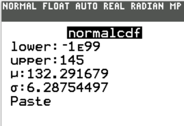
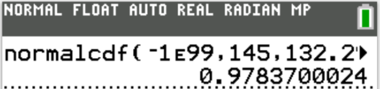
...will not be able to jump a height of 145 cm means that the child can jump less than 145 cm
Let us convert the height to a z-score
$ z = \dfrac{x - \mu}{\sigma} \\[5ex] z = \dfrac{145 - 132.291679}{6.28754497} \\[5ex] z = 2.021189679 \approx 2.02 \\[3ex] P(X \lt 145) = P(z \lt 2.02) = 0.97831 \\[3ex] $ (c.) a height of more than 135cm
at least 2 means ≥ 2
The complement is: < 2
Let:
x = random variable denoting the number of children who can jump more than 135 cm
p = probability of success
q = probability of failure
n = sample size
C(n, x) = number of combinations of n children taking x children at a time
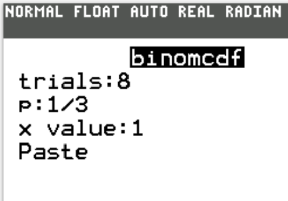
$ P(x) = C(n, x) * p^x * q^{n - x} \\[3ex] C(n, x) = \dfrac{n!}{(n - x)!x!} \\[5ex] n = 8 \\[3ex] P(X \gt 135) = p = \dfrac{1}{3} \\[5ex] q = 1 - \dfrac{1}{3} = \dfrac{2}{3} \\[5ex] P(x \ge 2) = 1 - P(x \lt 2)...\text{Complementary Rule} \\[3ex] P(x \lt 2) = P(x = 0) + P(x = 1) \\[5ex] P(x = 0) = C(8, 0) * \left(\dfrac{1}{3}\right)^0 * \left(\dfrac{2}{3}\right)^{8 - 0} \\[5ex] = \dfrac{8!}{(8 - 0)! * 0!} * 1 * \left(\dfrac{2}{3}\right)^8 \\[5ex] = \dfrac{8!}{8! * 1} * \dfrac{2^8}{3^8} \\[5ex] = \dfrac{256}{6561} \\[5ex] P(x = 1) = C(8, 1) * \left(\dfrac{1}{3}\right)^1 * \left(\dfrac{2}{3}\right)^{8 - 1} \\[5ex] = \dfrac{8!}{(8 - 1)! * 1!} * \dfrac{1}{3} * \left(\dfrac{2}{3}\right)^7 \\[5ex] = \dfrac{8!}{7! * 1} * \dfrac{1}{3} * \dfrac{2^7}{3^7} \\[5ex] = \dfrac{8}{3} * \dfrac{128}{2187} \\[5ex] = \dfrac{1024}{6561} \\[5ex] P(x \lt 2) = \dfrac{256}{6561} + \dfrac{1024}{6561} \\[5ex] P(x \lt 2) = \dfrac{1280}{6561} \\[5ex] P(x \ge 2) = 1 - \dfrac{1280}{6561} \\[5ex] P(x \ge 2) = \dfrac{6561}{6561} - \dfrac{1280}{6561} \\[5ex] P(x \ge 2) = \dfrac{5281}{6561} $
(a.)
(b.)
(c.)
The travel bus can hold 46 students.
Historically, 87% of students have shown up for the trip.
Using your knowledge of Statistics, how many tickets for the trip would you recommend the University Ski Club sells?
State your assumptions.
Show your calculations.
State your conclusions.
Give evidence to support your conclusions considering any costs and potential reputational effects.
Student: So, Mr. C, let me get this straight.
The bus can seat 46 students.
Teacher: Yes
Student: If they sell 46 tickets, will they make any loss?
Teacher: Apprently, no...because the cost of the ticket is set to a value that enables the club to make a profit.
Student: Why not just sell only 46 tickets?
Teacher: Well...it's the human being
Human beings are generally not content... we always want more
We are never satisfied.
The club has noticed over the years that some students who buy tickets do not show up.
So, they want to generate more revenue (make more money).
Hence, they want to see more tickets than the number of seats.
In other words, they do not want any lost revenue on empty seats.
Student: Okay, 87% historically show up
Hence, they want to take advantage of previous data and sell more tickets.
Teacher: That is correct.
Student: But what if they see more than 46...say they sell 55 tickets and all 55 students show up?
Does it mean that they will turn some students away?
Teacher: Or they can just order a minibus/minivan that would seat those extra students
In the context of the question, however, only one bus is assumed.
If they turn the extra students away, that is a reputational damage to the club.
Social media will not be nice to the club.
Hence, we want to avoid that.
Be it as it may, we want to assume that the 87% of students typically show up is correct.
Student: This implies that the probability that a student who buys a ticket show up is 87%.
Teacher: Yes...
So, what type of probability distribution should we use for this question?
Student: Based on only this question, I would say...Binomial Distribution
Even though the number of trials is large ...the computation using formulas is very big
Teacher: I understand.
Rather than use formulas, use a calculator or statistical software.
Student: What if we use a normal approximation to a binomial?
and apply the continuit correction?
Teacher: Approximating the binomial distribution with a normal distribution is useful for quick estimates and if statistical computations of the binomial distribution is not available.
Student: But it meets the conditions:
$ n = 46 \ge 30 \\[3ex] p = 87\% = 0.87 \\[3ex] q = 1 - 0.87 = 0.13 \\[3ex] np = 46(0.87) = 40.02 \gt 5 \\[3ex] nq = 46(0.13) = 5.98 \gt 5 \\[3ex] $ Teacher: I understand
But this scenario(question) is more suited for a binomial distribution
You can do both and compare/contrast the results
Binomial Distribution versus Normal Approximation to Binomial Distribution
Let's go ahead and do the Binomial Distribution.
Assumptions:
(1.) The scenario represents a Binomial Probability Distribution
Please see the reasons below.
(2.) The travel bus can hold 46 students.
The bus cannot take more than 46 students.
Only one bus is scheduled. There are no extra buses.
This implies that once the limit of 46 students is reached, any extra student will be turned away.
(3.) Historically, 87% of students have shown up for the trip.
This implies that based on previous data, 87% is assumed to be correct.
(4.) Based on historical data, the University Ski Club wants to generate extra revenue by preventing an lost revenue on empty seats.
Hence, we assume that they must sell more than 46 tickets.
| Conditions for a Binomial Distribution | Applicable Condition in Context | |
|---|---|---|
| (1.) | Fixed number of trials |
The "trials" represent the number of tickets sold. This is a fixed predetermined value that is decided by the club. |
| (2.) | For each trial, there are two possible outcomes: Success and Failure |
For every student who buys the ticket, there are two possibilities: The student shows up for the trip: Success The student does not show up for the trip: Failure |
| (3.) | Independent trials |
The decision of any student who buys the ticket to show up for the trip, or not show up for the trip
is assumed to be an independent decision. Let's assume that each student who buys a ticket makes an independent decision to show up or not show up for the trip. No external factors affect the decision. |
| (4.) |
Constant Probability of Success Let the probability of success = p The probability of success in one trial is the same as the probability of success in all the trials. Constant Probability of Failure Let the probability of failure = q The probability of failure in one trial is the same as the probability of failure in all the trials. |
The probability of success is the probability that a student who buys a ticket shows up for the trip.
$p = 87\% = \dfrac{87}{100} = 0.87$ The probability of success is the same for every student. No student who buys a ticket is more favored to show up for the trip more than any other student who purchased a ticket. The probability of failure is the probability that a student who buys a ticket does not show up for the trip. $ q = 1 - 0.87...\text{Complementary Rule} \\[3ex] q = 0.13 \\[3ex] $ The probability of failure is the same for every student. No student who buys a ticket is less favored to show up for the trip more than any other student who purchased a ticket. |
Calculations
All calculations and summaries are based on the historical 87% probability of success (probability that a student will show up for the trip after buying a ticket)
Let the:
Number of trials = Number of tickets = n
Number of students who show up = X
1st: Number of Tickets based on Complete Attendance Based on historical success rate of 87% show-up, how many tickets should be sold if 46 seats is filled?
$ \text{Assume 46 seats are filled} \\[3ex] \text{Expected Attendance based on historical data of 87%} \\[3ex] \text{How many tickets should be sold?} \\[3ex] 87\% * n = 46 \\[3ex] 0.87 * n = 46 \\[3ex] n = \dfrac{46}{0.87} \\[5ex] n = 52.87356322 \\[3ex] n \approx 53\;tickets \\[3ex] $ More than 46 tickets and Less than 53 tickets must be sold.
Next, we have to do the calculations on Binomial Distribution
Let us determine the probability for these cases:
What is the probability that more than 46 students show up when:
(1.) 46 tickets are sold (tickets are sold at bus capacity): $P(X \gt 46) \text{ when } n = 46$
(2.) 47 tickets are sold: $P(X \gt 46) \text{ when } n = 47$
(3.) 48 tickets are sold: $P(X \gt 46) \text{ when } n = 48$
(4.) 49 tickets are sold: $P(X \gt 46) \text{ when } n = 49$
(5.) 50 tickets are sold: $P(X \gt 46) \text{ when } n = 50$
(6.) 51 tickets are sold: $P(X \gt 46) \text{ when } n = 51$
(7.) 52 tickets are sold: $P(X \gt 46) \text{ when } n = 52$
We do not need to calculate the probability for every case.
We want to keep the probability that more than 46 students show up as small as possible.
We will stop when the probability is at least 5%.
5% is statistically significant in this case to minimize or avoid lost revenue and prevent reputational damage.
We chose 5% because it is a conventional cutoff for determining whether a result is statistically significant in hypothesis testing.
The formula for the Binomial Probability Distribution is: $P(x) = \dfrac{n!}{(n - x)! x!} * p^x * q^{n - x}$
However we shall not use the formula. We shall use a graphing calculator.
$ p = 0.87 \\[3ex] q = 0.13 \\[3ex] $ Case 1: 46 tickets are sold (tickets are sold at bus capacity)
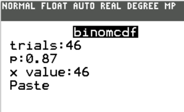
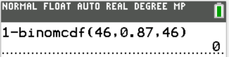
$ n = 46 \\[3ex] P(X \gt 46) = 0 \\[3ex] $ The probability that more than 46 students show up when 46 tickets are sold is 0.
This is the safest scenario.
Reputation is not damaged.
There are no losses because 46 tickets were sold.
Expected number of students to show up = $0.87(46) = 40.02 \approx 41...\text{rounded up}$
Estimated empty seats = $46 - 41 = 5$ seats.
However, there is lost revenue because seats are not filled.
Case 2: 47 tickets are sold
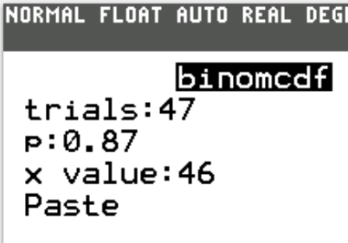
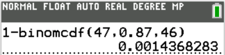
$ n = 47 \\[3ex] P(X \gt 46) = 0.0014368283 \\[3ex] $ The probability that more than 46 students show up when 47 tickets are sold is 0.0014368283 (≈ 0.14% to 2 decimal places)
This is a safe scenario because the probability is very low.
Expected number of students to show up = $0.87(47) = 40.89 \approx 41...\text{rounded up}$
There is extra revenue from the sale of 1 extra ticket.
Reputation is not damaged.
Estimated empty seats = $46 - 41 = 5$ seats.
However, there is lost revenue because seats are not filled.
Case 3: 48 tickets are sold
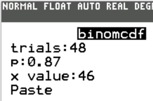
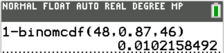
$ n = 48 \\[3ex] P(X \gt 46) = 0.0102158492 \\[3ex] $ The probability that more than 46 students show up when 48 tickets are sold is 0.0102158492 (≈ 1.02% to 2 decimal places)
This is a safe scenario because the probability is low.
Expected number of students to show up = $0.87(48) = 41.76 \approx 42...\text{rounded normal}$
There is extra revenue from the sale of 2 extra tickets.
Reputation is not damaged.
Estimated empty seats = $46 - 42 = 4$ seats.
However, there is lost revenue because seats are not filled.
Case 4: 49 tickets are sold
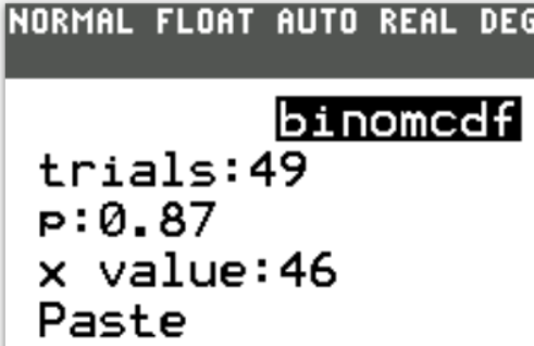
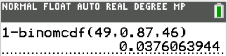
$ n = 49 \\[3ex] P(X \gt 46) = 0.0376063944 \\[3ex] $ The probability that more than 46 students show up when 49 tickets are sold is 0.0376063944 (≈ 3.76% to 2 decimal places)
This is an okay scenario because the probability is small.
Expected number of students to show up = $0.87(49) = 42.63 \approx 43...\text{rounded normal}$
There is extra revenue from the sale of 3 extra tickets.
Reputation is not damaged.
Estimated empty seats = $46 - 43 = 3$ seats.
However, there is lost revenue because seats are not filled.
Case 5: 50 tickets are sold
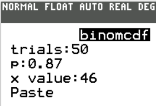
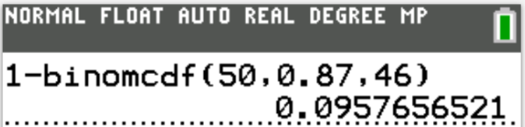
$ n = 50 \\[3ex] P(X \gt 46) = 0.0957656521 \\[3ex] $ The probability that more than 46 students show up when 50 tickets are sold is 0.0957656521 (≈ 9.58% to 2 decimal places)
This is not safe because the probability is more than 5%.
Expected number of students to show up = $0.87(50) = 43.5 \approx 44...\text{rounded normal}$
Even though the expected number is less than 46, the probability is a major concern.
If at least one of the 4 students show up and is turned away, the reputation of the club is questionable.
Conclusions
(1.) Based on the historiacal data, assumptions, and calculations, I recommend that the University Ski Club sell 49 tickets.
(2.) If 49 students buy tickets, the probability that more than 46 people will show up is 0.0376063944. This is an acceptable probability in this context. There is a low chance of turning any student away.
(3.) If 49 tickets are sold, about 43 students are expected to show up. That would leave about 3 seats unfilled which is lost revenue, however, the loss in revenue is not comparable/measurable to the damage in reputation the club will face if any student is turned away due to overbooking. To balance the generation of revenue with avoiding or minimizing reputational damage, 49 tickets should be sold.
(4.) In the event that 49 tickets are sold and more than 46 students show up, the club should make an apology to the affected student(s), and offer refunds and a convenience gift (a gift card, meal ticket or the like) accordingly.
(5.) To avoid turning away any student, the club should sell 46 tickets and have a waitlist of students that will replace the no-shows on a first-come, first-served basis.
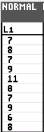
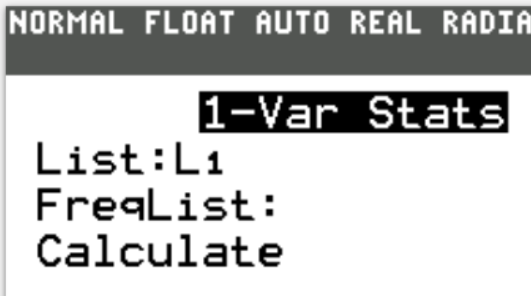
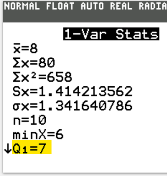
$ 7, 8, 7, 9, 11, 8, 7, 9, 6, 8 \\[3ex] \text{sample size, } n = 10 \\[3ex] \text{sort in ascending order: } 6, 7, 7, 7, 8, 8, 8, 9, 9, 11 \\[3ex] \text{confirm the sample size: } n = 10 \\[3ex] \text{1st Quartile, }Q_1 \\[3ex] = \dfrac{n}{4}th \\[5ex] = \dfrac{10}{4}th \\[5ex] = 2.5th \\[3ex] = 3rd \text{ value in sorted dataset...rounded up because 2.5 is a decimal} \\[3ex] = 7 \\[3ex] Q_1 = 7 $
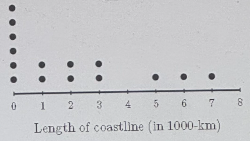
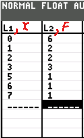
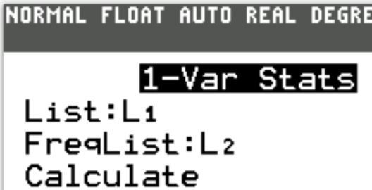
In the given dot plot, the length of the coastline of each country in South America is shown in thousands of kilometers (1000-km), rounded to the nearest thousand kilometers.
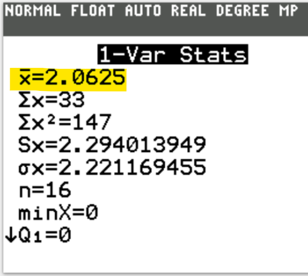
According to the dot plot, what is the mean length of coastline, in thousands of kilometers?
| Coastline Length (1000-km), $x$ | Frequency, $F$ | $Fx$ |
|---|---|---|
| 0 | 6 | 0 |
| 1 | 2 | 2 |
| 2 | 2 | 4 |
| 3 | 3 | 9 |
| 5 | 1 | 5 |
| 6 | 1 | 6 |
| 7 | 1 | 7 |
| $\Sigma F = 16$ | $\Sigma Fx = 33$ | |
| $ Mean, \bar{x} = \dfrac{\Sigma Fx}{\Sigma F} \\[5ex] = \dfrac{33}{16} \\[5ex] = 2.0625 \text{ thousand kilometers} \\[3ex] \approx 2\text{ thousand kilometers}...\text{to the nearest thousand kilometers}. $ | ||
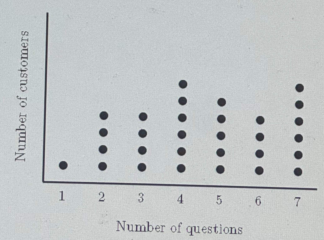
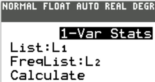
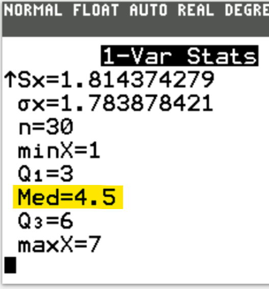
Judah, a marketing consultant, tracked how many times his customers asked a question during his sales calls over a one month period.
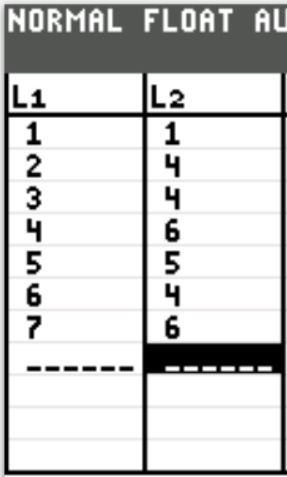
Based on the results shown in the distribution, what was the median number of questions asked?
| Number of Questions, $x$ | Number of Customers (Frequency), $F$ |
|---|---|
| 1 | 1 |
| 2 | 4 |
| 3 | 4 |
| 4 | 6 |
| 5 | 5 |
| 6 | 4 |
| 7 | 6 |
| $\Sigma F = 30$ | |
| $ \dfrac{\Sigma F}{2} = \dfrac{30}{2} = 15 \\[5ex] \underline{\text{From the top}} \\[3ex] 1 + 4 = 5 \\[3ex] 5 + 4 = 9 \\[3ex] 9 + 6 = 15 ...\text{Stop}...x = 4 \\[5ex] \underline{\text{From the bottom}} \\[3ex] 6 + 4 = 10 \\[3ex] 10 + 5 = 15 ...\text{Stop}...x = 5 \\[5ex] \text{Median number of questions asked} \\[3ex] = \dfrac{4 + 5}{2} \\[5ex] = 4.5 \\[3ex] \approx 5\text{ questions asked...to the nearest whole number}. $ | |
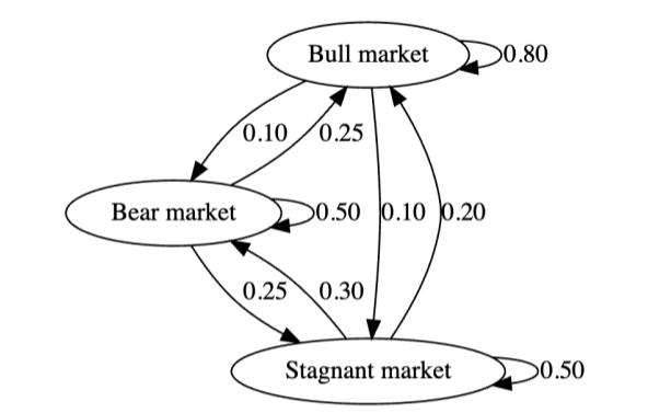
(a.) What is the transition matrix, T for this dynamical system?
Use the following ordering for the rows and columns: Bull market, Bear market, Stagnant market.
(b.) In the steady state, what is the probability of:
a bull market?
a bear market?
a stagnant market?
Based on the ordering: Bull market, Bear market, Stagnant market; we take the transition matrix as a column-stochastic matrix (left-stochastic matrix): $ \begin{bmatrix} \text{Bull} & \text{Bear} & \text{Stochastic} \end{bmatrix} $
This implies $ \begin{bmatrix} \text{Bull to Bull} & \text{Bear to Bull} & \text{Stagnant to Bull} \\[3ex] \text{Bull to Bear} & \text{Bear to Bear} & \text{Stagnant to Bear} \\[3ex] \text{Bull to Stagnant} & \text{Bear to Stagnant} & \text{Stagnant to Stagnant} \end{bmatrix} $
$ (a.) \\[3ex] T = \begin{bmatrix} 0.80 & 0.25 & 0.20 \\[3ex] 0.10 & 0.50 & 0.30 \\[3ex] 0.10 & 0.25 & 0.50 \end{bmatrix} $
Let the probability of a: Bull market, Bear market, Stagnant market in the steady state be A, B, C respectively.
The probability distribution, P can be represented as a column vector (column matrix) as $ \begin{bmatrix} A \\[3ex] B \\[3ex] C \end{bmatrix} $
(1.) In the steady state, $T * P = P$
(2.) The sum of the probabilities of the Bull market, Bear market, and the Stagnant market is 1.
$ \begin{bmatrix} 0.80 & 0.25 & 0.20 \\[3ex] 0.10 & 0.50 & 0.30 \\[3ex] 0.10 & 0.25 & 0.50 \end{bmatrix} * \begin{bmatrix} A \\[3ex] B \\[3ex] C \end{bmatrix} = \begin{bmatrix} A \\[3ex] B \\[3ex] C \end{bmatrix} $
$ 0.8A + 0.25B + 0.2C = A \\[3ex] 0.8A + 0.25B + 0.2C - A = 0 \\[3ex] -0.2A + 0.25B + 0.2C = 0 \\[3ex] -20A + 25B + 20C = 0 \\[3ex] -4A + 5B + 4C = 0 ...eqn.(1) \\[5ex] 0.1A + 0.5B + 0.3C = B \\[3ex] 0.1A + 0.5B + 0.3C - B = 0 \\[3ex] 0.1A - 0.5B + 0.3C = 0 \\[3ex] A - 5B + 3C = 0 ...eqn.(2) \\[5ex] 0.1A + 0.25B + 0.5C = C \\[3ex] 0.1A + 0.25B + 0.5C - C = 0 \\[3ex] 0.1A + 0.25B - 0.5C = 0 \\[3ex] 10A + 25B - 50C = 0 \\[3ex] 2A + 5B - 10C = 0 ...eqn.(3) \\[5ex] A + B + C = 1 ...eqn.(4) \\[5ex] eqn.(1) + eqn.(2) \implies \\[3ex] -3A + 7C = 0 ...eqn.(5) \\[5ex] \text{From eqn.(4)} \\[3ex] B = 1 - A - C ...eqn.(6) \\[3ex] \text{Substitute for B in eqn.(2)} \\[3ex] A - 5(1 - A - C) + 3C = 0 \\[3ex] A - 5 + 5A + 5C + 3C = 0 \\[3ex] 6A + 8C = 5 ...eqn.(7) \\[5ex] 2 * eqn.(5) + eqn.(7) \implies \\[3ex] [2(-3A + 7C)] + [6A + 8C] = 2(0) + 5 \\[3ex] -6A + 14C + 6A + 8C = 0 + 5 \\[3ex] 22C = 5 \\[3ex] C = \dfrac{5}{22} \\[5ex] \text{From eqn.(5)} \\[3ex] -3A = 0 - 7C \\[3ex] A = \dfrac{7C}{3} \\[5ex] A = \dfrac{7}{3} * \dfrac{5}{22} \\[5ex] A = \dfrac{35}{66} \\[5ex] \text{Substitute for A and C in eqn.(6)} \\[3ex] B = 1 - A - C ...eqn.(6) \\[3ex] B = 1 - \dfrac{35}{66} - \dfrac{5}{22} \\[5ex] B = \dfrac{66}{66} - \dfrac{35}{66} - \dfrac{15}{66} \\[5ex] B = \dfrac{66 - 35 - 15}{66} \\[5ex] B = \dfrac{16}{66} \\[5ex] B = \dfrac{8}{33} \\[5ex] (b.) \\[3ex] \text{In a steady state, the probability of :} \\[3ex] \text{Bull market} = \dfrac{35}{66} \\[5ex] \text{Bear market} = \dfrac{8}{33} \\[5ex] \text{Stagnant market} = \dfrac{5}{22} $


